Dan Olner’s Data Dispatch
About
Dan Olner’s Data Dispatch
Categories
All
(9)
code
(4)
data
(1)
firms
(2)
geo
(2)
gumph
(1)
io
(1)
migration
(1)
modelling
(1)
ons
(3)
planning
(2)
segregation
(1)
teaching
(1)
training
(1)
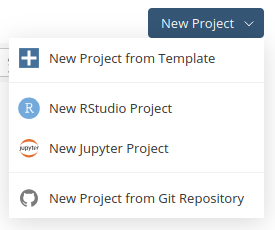
Getting started with using R and RStudio (in the cloud or on your own computer)
training
code
I’m running an “R + regional economic data” taster session in June. It won’t be necessary to use R during the session to follow along -
but if you want to have a go at…
May 16, 2025
Dan Olner
Data Stewards’ Network meeting on workflows
ons
data
I presented at a Sheffield University Data Stewards’ Network event, talking about the pipelines I’ve been building for ONS economic data and Companies House data (slides…
Mar 27, 2025
Dan Olner
Outputs live list
planning
RegEconTools website. All of this work comes under the broad heading of “Open regional economic data and tools”; this website is where I’m collating as much of this work as…
Feb 12, 2025
Dan Olner
Open data and code used for ONS subnational data conference
code
ons
planning
Off the back of presenting at the ONS subnational data conference, this post collects the open data / code I used in the slides, as well as a few extra bits mentioned in…
Nov 10, 2024
Dan Olner
How to automate your way out of Excel hell & other ONS data wrangling stories (business demography edition)
code
ons
firms
I’ve been analysing the latest ONS business demography data (that ONS pull from the IDBR). It contains a tonne of great data on business births, deaths, numbers, ‘high…
Nov 5, 2024
Dan Olner
What this situation needs is another blog, said no-one ever
gumph
“Another blog! Thank the Gods! Blogging is so
now
, isn’t it?”
Nov 4, 2024
Dan Olner
Pub crawl optimiser
code
teaching
geo
Well maybe. Sheffield R User Group kindly invited me to wiffle at them about an R topic of my choosing. So I chose two. As well as taking the chance to share my pain in…
Dec 7, 2016
Dan Olner
Migration entropy
migration
modelling
segregation
One of the parts of my new job (both here and here) is a project examining how migration and a host of other spatial-economic and social things interact. This is awesome…
Jan 16, 2016
Dan Olner
UK trade flows
firms
geo
io
This is one of the fun things I coded up in the process of developing the last grant I worked on. I’ll explain a bit about it and then share some thoughts on whether it’s…
Nov 26, 2014
Dan Olner
No matching items