Jun 16, 2017 - A script for automating RMarkdown to Jekyll

Comments

I’m going to be making a little more of an effort to get some coding up on this blog - not least because I’m always going, ‘now where’s that chunk of really useful code that does x and y?’ and having it here would make it easier for me to find.

So to start with, here’s something a little bit meta. I’ve been using RMarkdown on Windows to create blogposts for Jekyll, and part of that’s been using this little script to Knit the Post into jekyll-ready markdown.

So this post assumes you’re already doing something similar and know how to write in RMarkdown / copy the resulting Knitted posts and figures to your Jekyll site etc. At some point I need to write a full start-to-finish guide to doing this: it’s got a lot easier with some recent changes too. But for now, I just want to look at how to make the process smoother by automating some of the faff.

It might be things have moved on and there’s some much easier way of doing this internal to RStudio - do let me know if so!

The KnitPost function above creates the md file and also puts any figures in a folder in the local project. You then have to copy these to the correct place in your Jekyll folder - and also edit the header so it’s Jekyll-ready. Once you’ve done all that, you can preview locally using jekyll serve before pushing to the interwebs (as I’m doing here on my github.io site).

Which is great - but if you make an edit in your RmD, you have to then go through that process all over again. Mucho Fafferoo. I always have to make minor edits after I’ve posted something, as I suspect most people do: you don’t see a lot of errors or typos until you’re previewing and you’re bound to think of something you missed. Having to go through this faff each time? Harrumph.

So I’ve written an update to the above script that moves the files to the correct place once they’ve been created and replaces the header with the correct YML. This means you just need to write the thing, then call the KnitPost function, and can preview changes immediately.

The full function is below - just edit the URL of the Jekyll website and the path to your local Jekyll files.

And rather than load the function each time or package it up, I’ve just stuck mine into my Rprofile.site script so it’s loaded whenever RStudio runs. (I think I got that from here.) You’ll find the RProfile.site script in the Program folder of the R installation, in the ‘etc’ folder. (E.g. the path to mine is ‘C:\Program Files\R\R-3.3.0\etc’). Just copy/paste the function at the end of the script.

Then you can just write your RMarkdown script and run:

KnitPost('nameOfTheFile.Rmd','This is my lovely Jekyll article that will go to the right folder along with the figures')

The only little thing to note: it relies on there being three dashes to mark where to replace the header. By default, this is what RStudio creates if you make an Rmd script from its file menu. In theory it should be easy to code it to detect any number over three. I’ll leave that as an exercise for the reader…

Right, this has nicely reminded me how this whole Jekyll blog thing works. Now let’s start getting some less meta topics up here. Bye for now!

#~~~~~~~~~~~~~~~~~~~~~~~~~~~~~~~~~~~~~~~~~~~~~~~~~~~~~~~~~~~~~~~~~~~~~~~~
#Jekyll knitpost function
#~~~~~~~~~~~~~~~~~~~~~~~~~~~~~~~~~~~~~~~~~~~~~~~~~~~~~~~~~~~~~~~~~~~~~~~~
 
  #Input should be the name of the Rmd file (won't need path if it's in your project)
  KnitPost <- function(input, articleName = NULL) {
  
    #Adapted from 
	  #http://gtog.github.io/workflow/2013/06/12/rmarkdown-to-rbloggers/
    
    #Change to your site
    base.url <- c("http://danolner.github.io/")
    
    #Move the md file and figures here (to appropriate folders) after the knit process
    #Needs doing afterwards to avoid wrong path.
    myjekyllpath = 'C:/localpathtoyourjekyllsite'
    
    #Final article name
    #use filename if not included
    if(is.null(articleName)){
      articleName <- sub(".Rmd$", "", basename(input))
    } 
    
    #so you're not creating the fig folder every time
    ifelse(!dir.exists(file.path('figs')), dir.create(file.path('figs')), FALSE)
    
    require(knitr)
    opts_knit$set(base.url = base.url)
    fig.path <- paste0("figs/", sub(".Rmd$", "", basename(input)), "/")
    opts_chunk$set(fig.path = fig.path)
    opts_chunk$set(fig.cap = "center")
    render_jekyll()
    knit(input, envir = parent.frame())
    
    #~~~~~~~~~~~~~~~~~~~~
    #Make edits and moves----
    #Make matching folder if doesn't exist (we may be overwriting files but not the folder)
    targetdir <- c(paste0(myjekyllpath,'/figs/',sub(".Rmd$", "", basename(input))))
    
    ifelse(!dir.exists(file.path(targetdir)), 
           dir.create(file.path(targetdir)),FALSE)
    
    #http://stackoverflow.com/questions/10299712/copying-list-of-files-from-one-folder-to-other-in-r
    filestocopy <- list.files(path = paste0("figs/", sub(".Rmd$", "", basename(input)), "/"),
                              full.names = T)
    
    #Move figure outputs to jekyll folder
    file.copy(from=filestocopy, to=targetdir, 
              overwrite = T, recursive = FALSE, 
              copy.mode = TRUE)
    
    #~~~~~~~~~~~~~~~~~~~~~~~~~~~~~~~~~~~~~~~~~
    #Edit .md file to have jekyll-ready header----
    md <- readLines(paste0(sub(".Rmd$", ".md", basename(input))))
    
    #remove first line
    md <- md[2:length(md)]
    
    current <- md[1]
    
    while (current!='---') {
      #slice off the top
      md <- md[2:length(md)]
      current <- md[1]
      
    }
    
    #Then remove that line too once while done
    #(No do-while)
    md <- md[2:length(md)]
    
    #Add in jekyll header. This kinda structure
    # ---
    # layout: post
    # title: "testing again"
    # date: 2016-11-25
    # comments: true
    # ---
    theDate <- format(Sys.time(), "%Y-%m-%d")
    
    newHeader <- c(
      '---',
      'layout: post',
      paste0("title: \"", articleName,"\""),#this does work despite the output putting the escapes back in.
      paste0('date: ',theDate),#see ?date last example
      'comments: true',
      '---'
    )
    
    md <- c(newHeader,md)
    
    mdFileName <- paste0(myjekyllpath,
                         '/_posts/',
                         theDate,
                         '-',
                         gsub(' ','_',articleName),
                         '.md')
    
    #Ready to add to Jekyll folder
    writeLines(md,mdFileName)
    
  }
Dec 7, 2016 - Pub Crawl Optimiser

Comments

Spatial R for social good!

Well maybe. Sheffield R User Group kindly invited me to wiffle at them about an R topic of my choosing. So I chose two. As well as taking the chance to share my pain in coding the analysis for this windfarms project, I thought I’d bounce up and down about how great R’s spatial stuff is for anyone who hasn’t used it. It’s borderline magical.

So by way of introduction to spatial R, and to honour the R User Group’s venue of choice, I present the Pub Crawl Optimiser.

I’ve covered everything that it does in the code comments, along with links. But just to explain, there were a few things I wanted to get across. (A lot of this is done better and in more depth at my go-to intro to spatial R by Robin Lovelace and James Cheshire.) The following points have matching sections in the pubCrawlOptimiser.R code.

  • The essentials of spatial datasets: (in ‘subset pubs’) - how to load or make them from points and polygons, how to use one to easily subset the other using R’s existing dataframe syntax. How to set coordinate reference systems and project something to a different one, so everything’s in the same CRS and will happily work together. (The Travel to Work Area shapefile is included in the project data folder.)

  • Working with JSON and querying services: a couple of examples of loading and processing JSON data using the jsonlite package, including asking google to tell us the time it takes between pubs - accounting for hilliness. This is very important in Sheffield if one wants to move optimally between pubs. Pub data is downloaded separately from OpenStreetMap but we query OSM directly to work out the centroids of pubs supplied as ways.

  • A little spatial analysis task using the TSP package to find shortest paths between our list of pubs - both for asymmetric matrices with different times depending on direction, and symmetric ones just using distance.

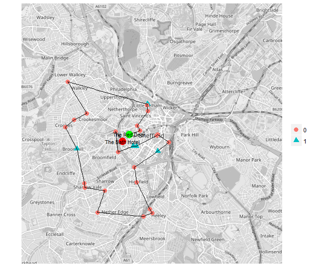
  • Plotting the results using ggmap to get a live OSM map for Sheffield. Note how easy it is to just drop TSP’s integer output into geom_path’s data to plot the route of the optimal pub crawl.

  • There’s also a separate script looking at creating a spatial weights matrix to examine spatial dependence. These are easy to create and do very handy jobs with little effort - e.g. if we want to know what the average number of real ale pubs per head of population in neighbouring zones, it’s just the weights matrix multiplied by our vector of zones.

The very first part of code that’s processing pub data downloaded from OSM - couple of things to note:

  • Just follow the overpass turbo link via the pub tag wiki page.
  • I remove the relations line ( relation[“amenity”=”pub”](); ) just to keep nodes and ways.
  • Once you’ve selected an area and downloaded the raw JSON, the R code runs through it to create a dataframe of pubs, keeping only those with names. It also runs through any that are ways (shapes describing the pub building), finds their points and averages them as a rough approximation of those pubs’ point location. I could have selected a smaller subset of data right here, of course, but wanted to show a typical spatial subsetting task.

A couple of friends have actually suggested attempting the 29 pub crawl in the code (below, starting at the Red Deer and ending at the Bath Hotel). I am not sure that would be wise.

So what would you want to see in an essential introduction to spatial R for anyone new to it?

Dec 7, 2016 - Introduction to data wrangling n viz in R

Comments

Introduction to R

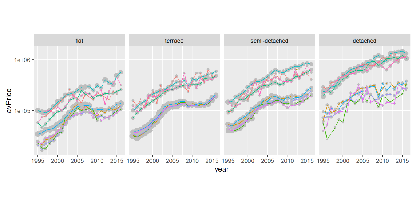
I just ran an introduction-to-R one day workshop here at the Sheffield Methods Institute on behalf of AQMeN. The aim was to introduce people with no previous experience of R to RStudio, data wrangling with the various tidyverse libraries and outputting some plots/visualisations with ggplot.

I’ll be updating the course based on experience of this first one, but if you want a go, the course booklet is written assuming no previous knowledge and should, in theory, work for self-learning. It’s all based on open access data so it’s available to everyone. If you’re interested:

  • go pick a city from here. Each is a zipped up RStudio project with that city/town’s travel-to-work area plus London.

  • Make sure you’ve got RStudio and R installed.

  • Look in the course_materials folder of your unzipped RStudio project: there’s a PDF there (and an HTML doc) with the course in. (Or the HTML one is online here.) It’ll explain how to open it in RStudio and get going.

The booklet runs through a typical data wrangling scenario using Land Registry ‘price paid’ data: a record of every property sale in England and Wales since 1995. It also does some data linkage, getting geographies from Ordnance Survey Code-Point Open data that gives precise locations for Great Britain postcodes. (CodePoint Open is some way down the list on that page.)

Any comments/suggestions, do let me know (d dot older at sheffield dot ac dot uk).

  • Note: the course uses data I’ve already got into a rather more useable form, to keep the focus on the essentials. If you want to know how to get from the original downloaded data, take a look at the preparation code. Though it ain’t pretty… which in itself is salutory: writing this stuff up can present a sanitised version of coding reality that appears way more ordered than it really is.

  • Note note: the full data prep code includes an explanation of how the postcodes were used to geocode geographies into a lookup, so serve as a real-data intro to geocoding in R. This code uses two (also open access) zone shapefiles: Travel-to-work areas (TTWAs) and ward shapefiles for England from the Census Edina boundary data download site. (TTWAs are in ‘England / Other / 2001-2010, wards are from England / Census / English Census Merged Wards 2011.)

center