Using R to wrangle data from web to output: ONS Local taster session (27th Nov 2025)

Before we start…

You’ve got two ways to engage with this session:

Just watch the screencast, let it wash over you and then come back to the materials in your own time. (These slides as well as ONS recording.)
Run the R code yourself as we go. If you’re trying #2 - you’ll need a copy of these slides open. You’ll have got the link via email - it’s also in the chat, or just type bit.ly/rpipelines into your browser address bar.

Navigate the slides with the up/down or left/right keyboard arrows.
Each slide is numbered - I’ll say where we’re at as we progress.
Note the three-bar button, bottom left - that lets you see the table of contents

One more chance to open your own slide copy! Get them at bit.ly/rpipelines.

Getting set up using R online (if you haven’t got R yet and want to)

Not got R yet?

If you want to do some coding but didn’t have a chance to run through the little R setup guide, you’ve got some time now while I do all the pre-amble.
The next slide takes you through how to get RStudio working in the browser using (free) posit.cloud.
I’ve also stuck an image of the ‘set up posit.cloud’ slide in the chat, if useful.

Get up and running with RStudio in the cloud

Use this link (or type bit.ly/positlogin into the address bar) to create an account at posit.cloud, using the ‘don’t have an account? Sign up’ box. It’ll ask you to check your email for a verification link so do that before proceeding.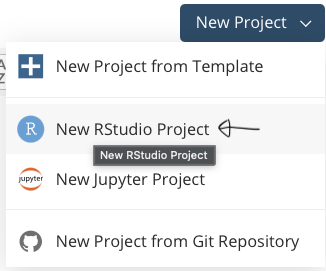
Once verified, go back to the posit.cloud tab and log in. You should see a message: “You are logged into Posit. Please select your destination”. Choose ‘Posit Cloud’ (not Posit Connect Cloud). That’ll take you to your online workspace.
Click the new project button, top right
Select ‘New RStudio project’ (as in the pic below). This will get us the latest available R version.

To give you a chance to get that set up…

Let me talk through some other bits:

We’ll use the free version of posit.cloud - it’s only got 1GB RAM, so we can’t do some of the heavier stuff, but is perfect for an intro. The paid tier isn’t too expensive and is powerful enough for most work.
Apologies - if posit.cloud doesn’t work for any reason, we won’t have time during this session to troubleshoot via chat - but we can work out ways to offer support after, if that’s useful.

The plan

We’ll be building a simple pipeline: running through three examples of getting data from the web, processing it, visualising it and outputting it into a little Word report.
The system we’ll use for output is called Quarto: it can also make PDFs, online reports, websites, blogs, and slides like the ones you’re looking at. The Quarto link has loads of info.
We’re not doing any web-hosted output here: we could do a future session on integrating github into your workflow, but that’s a bit much for today.

Get up and running with RStudio in the cloud

It should take less than a minute to open an RStudio project for you.
The R version running will be visible top-right and should be R 4.5.2.
If if isn’t for any reason, you can just select that dropdown and change to R 4.5.2 now.

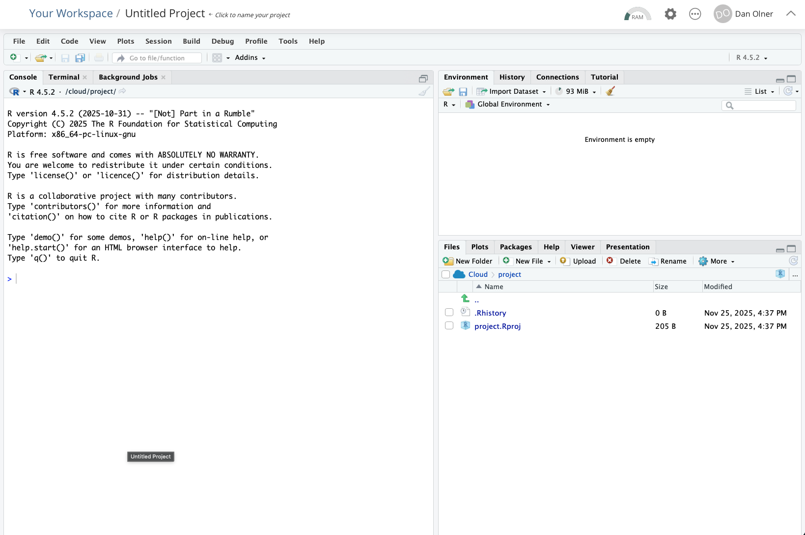
You should now see RStudio open, looking something like the pic below.

Copying code from these slides into RStudio

All code blocks here have a little clipboard symbol if you hover over them to quickly copy so you can paste it all into RStudio. This will come in especially handy with larger code blocks later…

2+2

[1] 4

sqrt(64)

[1] 8

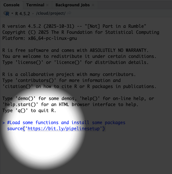
Task: run the setup code - copy and paste this line into the RStudio console and run it with ENTER

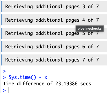
The first time this runs, it will install a couple of libraries/packages we need. It should take a bit less than two minutes to finish (it’ll tell you how long it took).

You can follow that link (or just go here) if you want to see what the code’s doing. We’re getting the tidyverse and NOMISR packages installed, and a couple of helper functions.

#Load some functions and install some packages
source('https://bit.ly/pipelinesetup')

Pasting into the console…

… should look something like this. Press enter to run, and then we wait for nearly two minutes.

(You’ll get some warning messages - don’t worry about those. If R breaks, it says ERROR not warning.)

That gives us another two minutes for me to waffle on…

These are methods I’ve been developing working with SYMCA, Yorkshire Universities and others as a Y-PERN policy fellow, seconded from Sheffield University. I’ve been compiling that work with all the open code here.
We’re now starting to use them to support other local authorities, and want to grow and improve these tools with collaboration/feedback from others
I’ve written a blog post on the rough plan, if of interest.

Sorry if things go wrong!

This is not a full training workshop. Whenever we’re learning new coding methods, things always go wrong, guaranteed. It’s all part of the fun.
If in a workshop, we can take time to fix those problems. Sorry, we won’t have capacity for that today.
The slides are designed to be step-by-step, and the session is being recorded by ONS - so you can work back through that in your own time.
But if you an actual supported workshop appeals, let me know: d.olner@sheffield.ac.uk

We’ll be running some chunky code blocks - especially if you’re new to R don’t worry about these making sense! Again - a workshop would be required to get into the detail.
The aim is just to run them in RStudio so you can get an idea of how this all works.
I will highlight a few key principles along the way, though.

How we’ll look at stuff

I’ve got two tabs open I’ll move between. 1: These slides with the code and links in. 2: RStudio, open in posit.cloud.
We’ll work through these slides together, sometimes typing or copying code from the slides into RStudio.

Given you’ll also have your own RStudio instance open, I’m aware this could be tricky!
So I’ll try to keep flitting about to a minimum: we’ll work in RStudio in big blocks, talking through the code using #codecomments to guide us.

One last thing - all the code for the Quarto output file is also online here, if you want to just get the whole thing rather than piece it together as we go.

Finally some coding?

Yep!

Assuming the setup code has now completed happily…

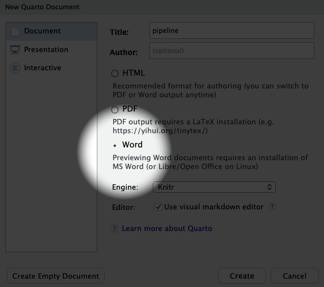
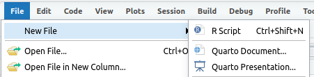
First job: we’re going to open the document that we’ll use to draft our output.
This is a ‘Quarto’ text file with the extension ‘qmd’

Task: open a new Quarto document

Use the file menu / new file and quarto document…

Task: open a new Quarto document

Add in a title, and choose the ‘Word’ option (noting the other options we’ve got here)

Task: try compiling the document

You’ll see RStudio has opened a quarto doc with some examples in.
Let’s just try compiling this, so you can see what happens. We’ll do exactly the same for our pipeline, just with more code in.
So: click on the Render button above the script.
You may see a warning, just cancel that.

The rendered document should now be in your RStudio project’s files

You can download that docx file by selecting its box and then choosing ‘export’ by clicking the little cog, top right (see pic).

Let’s start populating the Quarto doc

Task: copy this code and paste it just below ‘editor: visual’ in the quarto doc

This sets up some figure output choices and stops the doc from outputting all the R code and messages.

execute:
  echo: false
  message: false
  warning: false
fig-dpi: 300
fig-width: 8
fig-height: 5

Task: delete all the boilerplate code so we can start fresh

Just all the headings and code in the main part of the doc. We’ll be writing our own.

Task: then we add in our own setup code

To do this, let’s (1) make a new R code block (with code/insert chunk, see below - or use the shortcut)
Then (2) give it a name and (3) paste in the code below.
Don’t worry about the setup code: it won’t run for 2 minutes again. We just need it for some functions.

#Load some functions and install some packages
source('https://bit.ly/pipelinesetup')

library(tidyverse)
library(nomisr)
library(xml2)

#Set ggplot theme
theme_set(theme_light())

Once that’s done, we can just write some headings and text

Quarto has both a visual and source mode, for editing in different ways
‘Source’ shows the text file - we can add headings with hashes, or do in ‘Visual mode’ and use the formatting options

Let’s also add a heading in for our first web data import (something like ‘Extracting from an Excel file’)

Example one: extracting from an online Excel file

Task: now make another code block as we did before

This will be our first pipeline section. Once we’ve made it, we’ll add in the code below.
(Don’t worry about the code running off the slide below - it’ll still copy with the clipboard symbol.)

Here’s the code to copy into our new R code block:

# 1. Extracting from an Excel file on a website: productivity data example

# Copy the URL for the Excel sheet from the ONS website for subregional productivity data
# That's here:
# https://www.ons.gov.uk/employmentandlabourmarket/peopleinwork/labourproductivity/datasets/subregionalproductivitylabourproductivitygvaperhourworkedandgvaperfilledjobindicesbyuknuts2andnuts3subregions
# This is just setting a string named 'url'
url = 'https://www.ons.gov.uk/file?uri=/employmentandlabourmarket/peopleinwork/labourproductivity/datasets/subregionalproductivitylabourproductivitygvaperhourworkedandgvaperfilledjobindicesbyuknuts2andnuts3subregions/current/labourproductivityitls1.xlsx'

# We then create a TEMPORARY FILE...
temp_path = tempfile(fileext=".xlsx")
# And use that file path to DOWNLOAD A TEMP COPY OF THE EXCEL TO USE
download.file(url, temp_path, mode="wb")

# Or if you want to keep a local, month-dated version in case it changes later...
# download.file(
#   url,
#   paste0('ONS_outputperhourdata-',format(Sys.Date(),'%b-%Y'),'.xlsx'),
#   mode="wb")

# READ FROM THE EXCEL SHEET
# This goes straight into a dataframe
# Read directly from a specific sheet and range of cells from the downloaded file
# "Table A1: Current Price (smoothed) GVA (B) per hour worked indices; ITL2 and ITL3 subregions, 2004 - 2023"
cp.indices = readxl::read_excel(path = temp_path,range = "A1!A5:W247")

# TAKE A LOOK AT THAT DATA (CLICK ON ITS NAME IN THE ENVIRONMENT PANEL)
# It's got each year IN ITS OWN COLUMN. Not what we want.

# So we RESHAPE
# Get just ITL3 level and pivot years into their own column

# An aside: 
# This symbol - %>% 
# Is a PIPING OPERATOR
# It lets us pipe one operation to the next
# So we can clearly see each step taken
# Let's number those steps here

#1. Pipe the data into a filter
#2. filter down to just ITL3 zones
#3. pivot long so years are in their own column
#4. Convert year to a sensible format
#5. Remove the ITL column, we don't need that now
# And back on the first line, overwrite the original dataframe
cp.indices = cp.indices %>% 
  filter(ITL_level == 'ITL3') %>% 
  pivot_longer(Index_2004:Index_2023, names_to = 'year', values_to = 'index_value') %>% 
  mutate(
    year = substr(year,7,10),
    year = as.numeric(year)
  ) %>% 
  select(-ITL_level)


# We're going to plot JUST THE UK CORE CITIES
# Here's a list of those I made earlier...
corecities = readRDS(gzcon(url('https://github.com/DanOlner/RegionalEconomicTools/raw/refs/heads/gh-pages/data/corecitiesvector_itl3_2025.rds')))

# Check match...
# Note, this is commented out (so it doesn't output in our final doc)
# BUT we can still run it to check by highlighting the code
# table(corecities %in% cp.indices$Region_name)

# Plot!
# Filter down to the core cities
# And reorder the places by which has the highest average index over all years
ggplot(
    cp.indices %>% filter(Region_name %in% corecities),
    aes(x = year, y = index_value, colour = fct_reorder(Region_name,index_value,.desc = T))
    ) +
  geom_line() +
  geom_hline(yintercept = 100) +
  scale_color_brewer(palette = 'Paired') +
  theme(legend.title=element_blank()) +
  ylab('Output per hour: 100 = UK av')

That link to the Excel sheet in the code has been copied directly from the ONS subregional productivity webpage here…

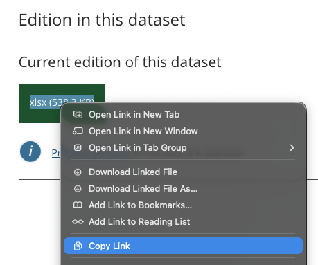
But you do need to do into the Excel file itself to look at what sheet and cell range you need. That only needs doing once though.

We’re going to use the very first sheet: A1, current prices smoothed.

Let’s move to RStudio to run through the first example

We can run each bit of the code inside the quarto doc (to make sure everything works as we want and see the outputs) as well as run the whole thing to compile the final doc.

Example two: using the NOMISR package to get data from NOMIS

We’re going to do something slightly different for this one

Often, getting the data wrangled can be time-consuming (due to either download or processing times)
We don’t want to have to go through that every single time the Quarto doc compiles.
One way to solve this: do the processing in a separate script, save it, then let the Quarto doc re-load the finished product.

Task: so let’s open a new R script in RStudio and do the NOMISR work there

In the file menu in RStudio
Use new file and R script (note: it tells you the keyboard shortcut for this)

Task: then we paste the NOMISR code below into our new script

And then let’s go through it in RStudio again

# Script to get NOMIS data via NOMISR package
# And then save for use in Quarto

# See https://docs.evanodell.com/nomisr/articles/introduction.html
# For NOMISR essentials

#Load some functions (and install some packages if not present)
source('https://bit.ly/pipelinesetup')

# Load libraries (if running for first time)
library(tidyverse)
library(nomisr)


# STEP 1: Get info on all available datasets
# Check how long... 14 seconds on my last attempt
x = Sys.time()

nomisinfo = nomis_data_info() %>% 
  select(id, description.value, name.value)

Sys.time() - x

# If that's being a pain or too slow
# Press the red STOP!! button and load this Blue Peter version
nomisinfo = readRDS(gzcon(url('https://github.com/DanOlner/RegionalEconomicTools/raw/refs/heads/gh-pages/bres_nomisdatasave.rds')))

# LET'S LOOK INSIDE THAT DATASET
# If we do that, we can search for the dataset code we want to use
# Let's search for 'employment' in RStudio...

# Now we can get metadata for the BRES data, having found the code
a = nomis_get_metadata(id = "NM_189_1")

#Pick on some of those for a closer look
#Note, MEASURE in the actual downloaded data is "MEASURE_NAME" column...

# We're going to use INDUSTRY PERCENTAGE
# to look at what percent of resident workers are in different sectors
# We'll use the code on the left
nomis_get_metadata(id = "NM_189_1", concept = "MEASURE")

# This one lists the employment type options we've got
nomis_get_metadata(id = "NM_189_1", concept = "EMPLOYMENT_STATUS")

# This one's especially useful - we need it to get the right geography code
geogz = nomis_get_metadata(id = "NM_189_1", concept = "GEOGRAPHY", type = "type")

print(geogz, n = 60)


# From the metadata, we're going to pull out the geography codes
# That we need to put into NOMISR
# for JUST the core cities again
# Slightly different names / shapes in BRES, but mostly the same
# Again, here's one I made earlier...
corecities.bres = readRDS(gzcon(url('https://github.com/DanOlner/RegionalEconomicTools/raw/refs/heads/gh-pages/data/corecities_bres.rds')))


# USE LOCAL AUTHORITIES TO GET ALL TIMEPOINTS
# ITL3 2021 zones in the BRES data only have 2022-2024
# "TYPE424 local authorities: district / unitary (as of April 2023)"
# Belfast won't be there cos BRES is GB but otherwise good
placeid = nomis_get_metadata(id = "NM_189_1", concept = "geography", type = "TYPE424") %>% 
  filter(label.en %in% corecities.bres) %>% select(id) %>% pull

# NOW WE GET THE ACTUAL DATA
# Using many of the codes we just looked at
# Check how long it takes too...

# p.s. if you want to save time, I've also Blue Petered this data
# You'll have the option to use that in the Quarto doc rather than run NOMISR

# I'm also not sure if the NOMIS API will be made sad by us all trying to download at the same time...

x = Sys.time()

# So the actual GET DATA function
# We pass in the various values we got from above
# Note also the option to set the year - we don't do that, so we get all of them
# We also select only some columns, which does save a bit of download time
bres = nomis_get_data(id = "NM_189_1",  geography = placeid,
                       # time = "latest",#Can use to get specific timepoint. If left out, we'll get em all
                       # MEASURE = 1,#Count of jobs
                       MEASURE = 2,#'Industry percentage'
                       MEASURES = 20100,#Just gives value (of percent) - redundant but lowers data download
                       EMPLOYMENT_STATUS = 2,#Full time jobs
                       select = c('DATE','GEOGRAPHY_NAME','INDUSTRY_NAME','INDUSTRY_TYPE','OBS_VALUE')
)

Sys.time() - x

# That takes 25-30 seconds in posit's R
# No fun if you're trying to check changes - don't want to run that every time
# Get the data in a different script and store somewhere the quarto doc can reload easily

# Save for use in quarto
# The RDS format is quick and compact
saveRDS(bres,'bres_nomisdatasave.rds')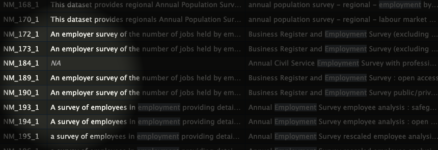

Looking for our dataset code in the NOMISR-downloaded catalogue

What it should look like / how long it’ll take downloading this data

OK, now we can get that NOMIS data into our output

Now it’s saved, that’s very straightforward - we reload the data we just saved.

Why does it need reloading into the Quarto script?

Because every time a Quarto doc is compiled, it starts with an empty environment, so no other data or libraries are visible to it.
This is a good thing: it means they have to be self-contained.

Task: make a new heading and code block in the Quarto doc and copy/paste this code in

We’ll then go through the code again.

# Get the BRES data we extracted in the separate script
bres = readRDS('bres_nomisdatasave.rds')

# Or load a 'here's one I made earlier' version if NOMISR wasn't playing for any reason
# bres = readRDS(gzcon(url('https://github.com/DanOlner/RegionalEconomicTools/raw/refs/heads/gh-pages/bres_nomisdatasave.rds')))

# Check its size in memory
#pryr::object_size(bres)

# Quick look at the data structure, filtered down to just 2 digit SICs
# bres %>% filter(INDUSTRY_TYPE == 'SIC 2007 division (2 digit)') %>% View

# WE CAN DO DATA CHECKS IN A QUARTO DOC
# I TEND TO COMMENT THEM OUT SO THEY DON'T OUTPUT BUT IT CAN BE USEFUL TO KEEP IT ALL TOGETHER.

# For instance:
# Check industry percentages sum to 100 per ITL3 zone
# Mostly - some roundings-down build up to not quite 100%
# bres %>%
#   filter(INDUSTRY_TYPE == 'SIC 2007 division (2 digit)') %>%
#   group_by(GEOGRAPHY_NAME,DATE) %>%
#   summarise(totalpercent = sum(OBS_VALUE))

# WE'LL PICK OUT JUST FINANCE SECTORS TO LOOK AT HOW JOB PROPORTIONS HAVE CHANGED OVER TIME
# Remember, we already filtered down to core cities to lessen the download

# OK, let's look at the three finance 2-digit sectors
# 2 digit SICS are 64,65 and 66: sum those
# Pick out just 2 digit first as well
finance.percent = bres %>% 
  filter(
    INDUSTRY_TYPE == 'SIC 2007 division (2 digit)',
    qg('64|65|66', INDUSTRY_NAME)
  ) %>% 
  group_by(GEOGRAPHY_NAME,DATE) %>% 
  summarise(
    percent = sum(OBS_VALUE)
  ) 

# Plot. May need to smooth
ggplot(
  finance.percent, 
  aes(x = DATE, y = percent, colour = fct_reorder(GEOGRAPHY_NAME,percent,.desc = TRUE))
  ) +
  geom_line() +
  scale_color_brewer(palette = 'Paired') +
  theme(legend.title=element_blank()) +
  scale_x_continuous(breaks = unique(finance.percent$DATE)) +
  ylab('Percent') +
  ggtitle('Percent jobs in finance sectors, GB core cities')


# While we're here, extract a single value from the data to use inline
edinburgh_latestpercent = finance.percent %>% 
  filter(
    DATE == max(DATE),
    GEOGRAPHY_NAME == 'City of Edinburgh'
    ) %>% 
  pull(percent)

Task: we can also add R code directly into the text - for instance, so we can add values from the data

Paste the following chunk in as text after the code block. Pasting into visual moded should work fine.

You can run code in the text too, to include dynamic values from the data, rather than handwriting those in. For instance, we can say that **the percent of Edinburgh's finance jobs in `r max(bres$DATE)` was `r edinburgh_latestpercent`%.**

Task: data can go straight into tables too

Paste the following into a new R code chunk - it’ll use the data to populate a table.

knitr::kable(
  finance.percent %>% 
    filter(DATE == max(DATE)) %>% 
    select(City = GEOGRAPHY_NAME, percent) %>% 
    arrange(desc(percent)), 
             # escape = FALSE, 
             caption = paste0("Table: core cities' percent of finance jobs in ",max(finance.percent$DATE)," (SICs 64-66)"))

3. Scraping links from a website and downloading zips

In the last example, we’ll look at how to grab all links from a site and download zips from it

Yes, it’s the NOMIS website - bulk Census 2021 data - but it works for any site.
I use this approach to download and process Companies House data, for example.
Here, we’re going to look at occupation data for core cities in England and Wales.

Here’s the NOMIS webpage we’re using

It’s the NOMIS bulk Census 2021 download page - if you open that, it’s got a range of zip files for different variables.
Looking on that site, we can see under ‘work and travel’ that occupation data has the code TS063…
Let’s grab the code and paste it into its own section…

Task: in the Quarto doc, start a new section, make a new code block and paste this in

# From NOMIS webpage bulk Census download
website_basename = "https://www.nomisweb.co.uk"

# We use the xml2 library to read the page
doc = read_html(paste0(website_basename,"/sources/census_2021_bulk"))

# Extract all <a> tags with hrefs containing "census2021*.zip"
zip_links = xml_attr(
  xml_find_all(doc, "//a[contains(@href, 'census2021') and contains(@href, '.zip')]"),
  "href"
)

#Set global timeout to very bigly indeed for parsing and downloading
#ten hours per file covers all eventualities!
options(timeout = 36000)

# AS WE'VE DONE BEFORE, WE DOWNLOAD A ZIP TO A TEMPORARY LOCATION
url = paste0(website_basename,zip_links[qg('TS063', zip_links)][1])
temp_path = tempfile(fileext=".zip")
download.file(url, temp_path, mode="wb")

# LOOK INSIDE ZIP FOLDER - We can see separate files for different geographical scales
# With list = TRUE, this DOES NOT unzip - it just lists the zip folder's contents
filenames = unzip(temp_path, list = TRUE)

# Take a look...
# filenames
# IT CONTAINS SEPARATE CSVS FOR DIFFERNT GEOGRAPHICAL SCALES
# We want lower tier local authorities
# Here's an explanation for Census geographies...
# https://www.ons.gov.uk/census/census2021dictionary/areatypedefinitions

# Pick the geographical scale we want
# HERE, UNZIP IS EXTRACTING A SPECIFIC FILE FROM INSIDE IT
# WITHOUT UNZIPPING THE WHOLE THING
occ = read_csv(unzip(temp_path, files = filenames$Name[qg('ltla',filenames$Name)]))

# TAKE A LOOK AT THE COLUMN NAMES FOR THAT DATA
# Again, we've got columns that we want to pivot
# colnames(occ)               
occ = occ %>% 
  pivot_longer(
    4:13, names_to = 'occupation', values_to = 'count'
  )


# We then keep just the subgroup occupations
# And find our own percentages for each place
occ = occ %>% 
  filter(
    !qg('all usual',occupation)
    ) %>%
  group_by(geography) %>% 
  mutate(
    percent_occ = (count / sum(count)) * 100
    ) %>% 
  ungroup()

# Confirm sums to 100% per place... tick
# occ %>% group_by(geography) %>% 
#   summarise(percentsum = sum(percent_occ))

# Nicer occupation names
occ = occ %>% 
  mutate(
    occupation = case_when(
      qg('Managers', occupation) ~ 'Managers, directors & senior officials',
      qg('Professional occ', occupation) ~ 'Professionals',
      qg('Associate', occupation) ~ 'Associate professional & technical',
      qg('secretar', occupation) ~ 'Admin & secretarial',
      qg('trades', occupation) ~ 'Skilled trades',
      qg('caring', occupation) ~ 'Caring, leisure & other service',
      qg('sales', occupation) ~ 'Sales & customer service',
      qg('process', occupation) ~ 'Process, plant & machine operatives',
      qg('elementary', occupation) ~ 'Elementary'
    )
  )

# Filter to core cities
# table(corecities %in% occ$geography)
# table(c(corecities,'Cardiff','Newcastle upon Tyne') %in% occ$geography)

# core city names from BRES will work for us here
# We lose Glasgow, Edinburgh and Belfast as it's England and Wales Census data
corecities.bres = readRDS(gzcon(url('https://github.com/DanOlner/RegionalEconomicTools/raw/refs/heads/gh-pages/data/corecities_bres.rds')))

occ.core = occ %>% 
  filter(
    geography %in% corecities.bres
  )


# Might a filled bar is the way forward? Hmm.
ggplot(
  occ.core,
  aes(y = geography, x = percent_occ, fill = occupation)
) +
  geom_bar(position="fill", stat="identity") +
  scale_fill_brewer(palette = 'Paired') +
  ylab("")

Task: that’s OK, but what about how those places compare to average?

Finishing up with using the same downloaded zip to get England and Wales data as a whole, to make a ‘how do core cities differ from average?’ plot
Grab the code… if we have time…

# Get occupation values for England outside London
# To compare differences
occ.all = read_csv(unzip(temp_path, files = filenames$Name[6])) %>% 
  filter(geography != 'London') %>% 
  pivot_longer(
    4:13, names_to = 'occupation', values_to = 'count'
  )

# Sum for rest of England/Wales outside London
# By occupation
occ.all = occ.all %>% 
  group_by(occupation) %>% 
  summarise(count = sum(count)) %>% 
  filter(!qg('usual',occupation)) %>% 
  mutate(percent_occ = (count/sum(count)) * 100)

occ.all = occ.all %>% 
  mutate(
    occupation = case_when(
      qg('Managers', occupation) ~ 'Managers, directors & senior officials',
      qg('Professional occ', occupation) ~ 'Professionals',
      qg('Associate', occupation) ~ 'Associate professional & technical',
      qg('secretar', occupation) ~ 'Admin & secretarial',
      qg('trades', occupation) ~ 'Skilled trades',
      qg('caring', occupation) ~ 'Caring, leisure & other service',
      qg('sales', occupation) ~ 'Sales & customer service',
      qg('process', occupation) ~ 'Process, plant & machine operatives',
      qg('elementary', occupation) ~ 'Elementary'
    )
  )

# Stick them all togeher into one dataframe
# Rows can go on the end, as long as we make sure structure is the same
occ.compare = bind_rows(
  occ.core %>% select(-date,-`geography code`),
  occ.all %>% mutate(geography = 'E+W minus London')
)


# Can now see how core cities differ from average (outside London)
ggplot() +
  geom_point(
    data = occ.compare %>% filter(!qg('e\\+w', geography)), 
    aes(x = percent_occ, y = occupation, colour = geography),
    size = 3,
    shape = 17
    # height = 0.1
    ) +
  scale_color_brewer(palette = 'Paired') +
  geom_point(
    data = occ.compare %>% filter(qg('e\\+w', geography)), 
    aes(x = percent_occ, y = fct_reorder(occupation,percent_occ)),
    size = 7, shape = 3, colour = 'black'
  ) +
  xlab('Occupation % of all employed (18+)') +
  ylab("") +
  ggtitle('Census 2021: core cities % occupations\nEng/Wales minus London % overlaid (cross)')

OK, we’re done

Hopefully some of that worked or made sense

If the final output didn’t work, for some reason, there’s a version to download here to have a look at what it should in theory have done!
Would a workshop on any of this stuff might be of interest?
The next logical step is something on using github as the repository for open output…