Get set up using R online, make a script in RStudio and run code from github

These slides run through 3 things:

  1. Getting set up using R and RStudio in posit.cloud through the browser. (See here if you want a run-through of setting up R on your own machine.)
  2. Getting started using RStudio - making a new script, entering some commands and loading a library.
  3. An example of grabbing code from github to run in RStudio online (jump here to skip R intro). The script you’ll grab is self-contained: all code and packages are included, and the #codecomments run you through its use. (In this example, we’ll make a GVA * jobs ‘block’ plot. See comments for details…)
  • RStudio in posit.cloud is free for the most basic version (1GB memory, 25 projects). That’s plenty for a lot of stuff. There are paid tiers too, if you want to do heavier things (and avoid all installing-R-on-work-machine pain).
  • With the free version, you get 25 ‘compute hours’ a month (which is calculated in a mildly confusing way but should be fine for occasional use).
  • Pricing for more compute power and time is pretty reasonable, if you end up wanting more.

1. Get R/RStudio running in your browser with posit.cloud

Get up and running with RStudio in the cloud

  • Use this link (or type bit.ly/positlogin into the address bar) to create an account at posit.cloud, using the ‘don’t have an account? Sign up’ box. It’ll ask you to check your email for a verification link so do that before proceeding.
  • Once verified, go back to the posit.cloud tab and log in. You should see a message: “You are logged into Posit. Please select your destination”. Choose ‘Posit Cloud’ (not Posit Connect Cloud). That’ll take you to your online workspace.
  • Click the new project button, top right
  • You can either select ‘new project from template’ and then “Data Analysis in R with the tidyverse” to get a tidyverse-ready RStudio. If you’re not sure, choose this one - we’ll run through loading the tidyverse below.
  • Or choose ‘New RStudio project’ if you want to start with a blank slate.

2. Using RStudio

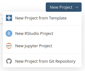
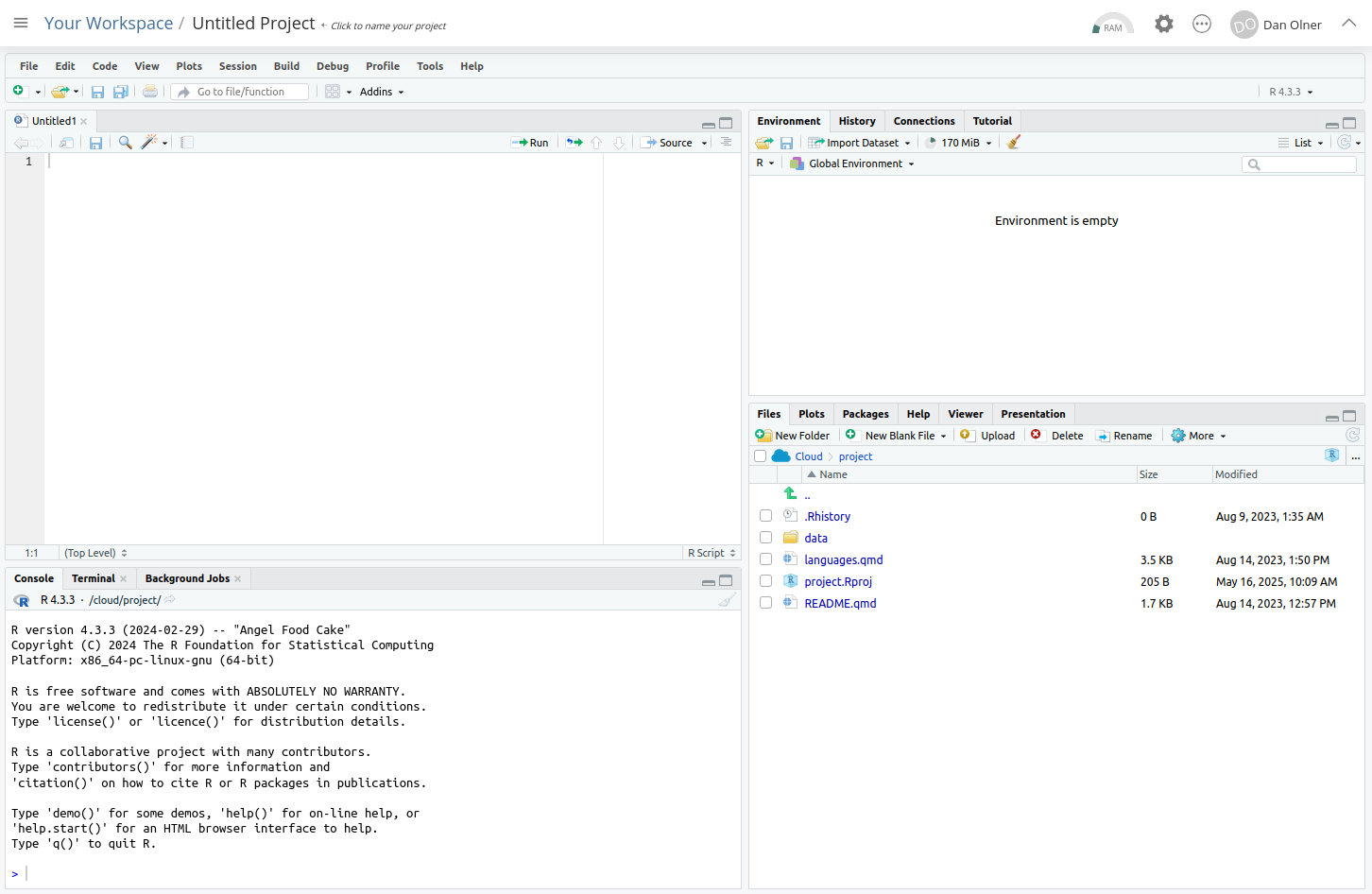
You should now have RStudio open in your posit.cloud account…

It should look something like the pic below.

Making a new R script in RStudio

RStudio is where you’ll be doing all the R loveliness.

Before looking at RStudio in more detail, let’s make a new R script, where you’ll do most of your coding.

Task: Open a new R script in RStudio

  • In the file menu in RStudio
  • Use new file and R script (note: it tells you the keyboard shortcut for this)

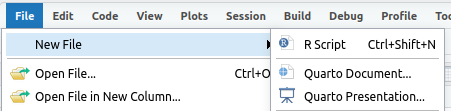
After that new file’s been made, the script will be open in RStudio, top left (see pic).

Tour of RStudio and essentials

1. The console

The console is bottom left: all R commands end up being run here. You either run code directly in the console or send code from your R script.

Task: enter some commands directly into the console

Click in the console area so the cursor is on the command line. Type some random sums (or copy, see next slide) - press enter and you’ll see the results directly in the console.

Note that second one: sqrt is a function and arguments go into the brackets. More on that in a mo.

2+2
[1] 4
sqrt(64)
[1] 8

Copying code from these slides into RStudio

All code blocks here have a little clipboard symbol if you hover over them (see pic) to quickly copy so you can paste it all into RStudio. Click on the clipboard to copy the text. This will come in especially handy with larger code blocks later…

2+2
[1] 4
sqrt(64)
[1] 8

2. Giving things names

We can assign all manner of things a name to then use them elsewhere: values, strings, lists - and, crucially, data objects like all the UK’s regional GVA. But these all use the same method.

Task: Still in the console, assign a value to a name

x = 64

You’ll see that assignment appear top right in RStudio. It can be retrieved just with:

x
[1] 64

3. Using an R script

We’ll now stick some code into that newly created R script we made earlier in the top left of RStudio.

All code will run in the console - what we do with scripts is just send our written/saved code to the console.

Let’s test this by adding code to load the tidyverse library.

What’s the tidyverse?

It’s a basket of tools that have become part of the R language - they all fit together to make consistent workflows much easier.

The online book R for Data Science is a great source to learn it, by the person who started it.

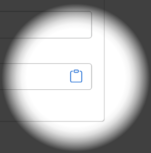
Task: add a line of code to the R script

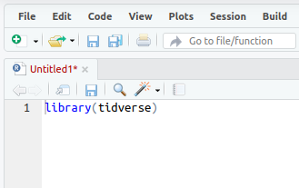
Type or paste the following text at the top of the newly opened R script in the top left panel.

library(tidyverse)

When you’ve put that in, the script title will go red, showing it can now be saved (it should look something like the image below).

  • Save the script either with the CTRL + S shortcut, or file > save. Give it whatever name you like, but note that it saves into your self-contained project folder.

Task: Run the library(tidyverse) line

Now we need to actually run that line of code… we can do this in a couple of ways:

  1. In your R script, if no code text is highlighted/selected RStudio will Run the code line by line (or chunk by chunk - we’ll cover that in the taster session).
  2. If a block of text is highlighted, the whole block will run. So e.g. if you select-all in a script and then run it, the entire script will run.

Let’s do #1: Run the code line by line.

  • To test this, we’ll load the tidyverse library with the code we just pasted in (which is just one line of code at the moment!) Put the cursor anywhere on the libary(tidyverse) line in the script (if it’s not there already), either with the mouse or keyboard. (Keyboard navigation is mostly the same as any other text editor like Word, but here’s a full shortcut list if useful.)
  • Once there, either use the ‘run’ button, top right of the script window, or (much easier if you’re doing this repeatedly) press CTRL+ENTER to run it.

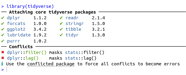
If all is well, you should see the text below in the console - the tidyverse library is now loaded. Huzzah!

3. Grabbing some code from github: a “GVA x Jobs blocks” example

Getting code from elsewhere into posit.cloud

  • We’ll look at an example of an R script that will run entirely self-contained in posit.cloud (if you’ve used the tidyverse template). It loads some GVA and jobs data and a geography lookup. On first run, it’ll install the ggrepel package for some better labels.
  • We’ll go to github and either download the code and import it into posit.cloud, or just copy-paste directly into an R script.
  • The code will plot GVA vs GVA-per-fulltime-job in sector blocks, stacked in order of productivity (gva per full time job). It can be a revealing way to look at productivity.
  • It’s done at ITL3 level, and we can select ITL3s within a particular ITL2 (e.g. West Yorkshire, South Yorkshire…)
  • Here’s a blog post talking through the data and resulting questions in a bit more detail.

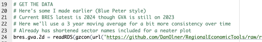
Task: Go to the github page where the code lives

  • Go to this github page to find the code. (That link will open in a new tab).
  • Look for the ‘raw’ options, top right. You’ve got a couple of choices here:
  1. The middle ‘copy raw file’ button: click this and github will stick the whole text onto the clipboard, ready for pasting into an R script - just as we did above with the single line of code.
  2. The right-hand ‘download raw file’ button: download a copy, and then use the upload button at the top of the files tab in RStudio to import it. It’ll then be in the file list - click on it to open.

If you’re pasting code from the clipboard…

  • Either make a new script again, as we did in this slide. It’ll open in a new tab.
  • Or just delete the code from your existing R script and paste into that.
  • Once that code is into an R script, we can run it chunk by chunk from top to bottom, as described in this slide earlier - run each code chunk by placing the cursor there and either using CMD/CTRL + ENTER or using the ‘run’ button.
  • Comments in the script talk through what each chunk is doing - the next couple of slides explain one or two key things.
  • You can also select all text with CTRL or CMD + A - and then CTRL/CMD + ENTER will run the whole thing in one go.
  • So: run all the first lines loading libraries (and installing ggrepel)
  • Then load the combined GVA and BRES jobs data (see pic)

  • You’ll know that’s run OK if bres.gva.2d has appeared in the environment panel - click anywhere on its name in that panel to view the data.

If you want different geographies

  • Then you’ll want to tweak the code the sets the listofplaces (from line 40). There are a couple of options.
  • Use the geog lookup that’s loaded in. You can get all ITL3 zones within e.g. the West Yorkshire ITL2 (this is the default). See pic - either set the name directly or use the grepl line to search for a partial match.

  • You’ve also got the option of setting the ITL3 name directly, either by a regex search or in a string - see the next few lines in the script for examples.
  • Then run the rest of the code to make the plot. It should look something like the example on the next slide. Picking out a couple of things to note:
  • Finance is fewer-jobs but large output (the area of the plot is total GVA) and large in all but one ITL3 here.
  • Note warehousing in Wakefield: many jobs, but average output per job is low.

View and save the plot

  • You may need to click on the ‘Plots’ panel to see the output.
  • Use the ‘Zoom’ option to pop out a resizeable view of the plot.
  • The final ggsave command in the script saves a copy as a png into the project’s folder. You can view and download it from there - use ‘Export’.

That’s all folks

Onto more R goodness!

Let me know if anything doesn’t work or doesn’t make sense - d dot olner at sheffield dot ac dot uk