Using R for regional economic analysis, ONS Local taster session (17th June 2025)

Before we start…

You’ve got two ways to engage with this session:

Just watch the screencast, let it wash over you and then come back to the materials in your own time. (These slides as well as ONS recording.)
Run the R code yourself as we go. If you’re trying #2 - you’ll need a copy of these slides open. You’ll have got the link via email - it’s also in the chat, or just type bit.ly/rtasterslides into your browser address bar.

If the slide link isn’t working for any reason, you’ll also have been sent a Word doc with the same material in

Not got R yet?

If you want to do some coding but didn’t have a chance to run through the little R setup guide, you’ve got some time now while I do all the pre-amble!
The slide below takes you through how to get RStudio working in the browser using (free) posit.cloud.
We’ll use the free version of posit.cloud - it’s only got 1GB RAM, so we can’t do some of the heavier stuff, but is perfect for an intro.
(The paid tier isn’t too expensive and is powerful enough for most work.)

I’ve also stuck an image of the ‘set up posit.cloud’ slide in the chat, if useful.
Sorry - if posit.cloud doesn’t work for any reason, we won’t have time during this session to troubleshoot via chat - but we’ll work out ways to offer support after, if that’s useful.
( Link to your own slide copy in the browser again, just in case: bit.ly/rtasterslides )

Get up and running with RStudio in the cloud

Use this link (or type bit.ly/positlogin into the address bar) to create an account at posit.cloud, using the ‘sign up’ box. It’ll ask you to check your email for a verification link so do that before proceeding.
Once verified, go back to the posit.cloud tab and log in. You should see a message: “You are logged into Posit. Please select your destination”. Choose ‘Posit Cloud’ (not Posit Connect Cloud). That’ll take you to your online workspace.
Click the new project button, top right
Select ‘new project from template’ (as in the pic below) and then “Data Analysis in R with the tidyverse” (if not already selected). Select then click OK down at the bottom. This will open your RStudio project where we’ll do the coding.

Introduction

We’ll be doing a whistlestop tour of using R for digging into UK regional economies.
For this session, we’re using just one ONS source - regional GVA broken down by industry. At the end I’ll list a bunch of other sources and ideas, and code for using them.
We’ll also be asking which of these would be most useful to you for future sessions, and what other data or tools might interest you.

These are methods I’ve been developing working with SYMCA as a Y-PERN policy fellow, seconded from Sheffield University. I’ve been compiling that work with all the open code here.
We’re now starting to use them to support other local authorities, and want to grow and improve these tools with collaboration/feedback from others.

Goals for the session

Actually get you started using R and RStudio if you haven’t used them before.
Give you a sense of how R can be used for UK regional data analysis and output.
Signpost to next steps if you want to do more. For anyone who does want to continue, I’m keen to grow our networks to collaborate on our capacity building.

I’ll also be banging on about how great R is for open, collaborative working. It’s build for openness and reproducibility, and this makes them great for collaborative learning.
I’ll talk about how to make reproducible pipelines all the way from data source to outputs.
The slides you’re looking at are an example: code available here.

Because this is just a taster session…

This is not a full training workshop. Whenever we’re learning new coding methods, things always go wrong, guaranteed. It’s all part of the fun.
If in a workshop, we can take time to fix those problems. Sorry, we won’t have capacity for that today.

Your options when things don’t work:
- The slides are designed to be step-by-step, and the session is being recorded by ONS - so you can work back through that in your own time.
- If you think fuller training where we can work through snags would be good, let’s work out how to make that happen. Get in touch.

We’ll take time at the start getting set up with RStudio so you have a foundation to work from.
But after that, we’ll be running some chunky code blocks - especially if you’re new to R don’t worry about these making sense! Again - a workshop’s required to get into the detail.
The aim is just to run them in RStudio so you can get an idea of how it works.
I will highlight a few key principles along the way, though.

The plan

I’ve got two tabs open I’ll move between. 1: These slides with the code and links in. 2: RStudio, open in posit.cloud.
We’ll work through these slides together, sometimes typing or copying code from the slides into RStudio.
Navigate the slides with the up/down or left/right keyboard arrows.
You can move between those two tabs, and also come back to Teams to see how I’m doing stuff.
Each slide is numbered - I’ll say where we’re at as we progress.

If you don’t fancy constantly flitting between slides and RStudio I’ve also made a single copy of the whole script we’ll work through that includes the slide text - I’ll show how to get that below at the point we’d stick it into RStudio.

One last thing…

Once you have your own copy of the slides open, note the three-bar button, bottom left.
That lets you see the table of contents

Also last chance to open own slide copy! Get them at bit.ly/rtasterslides.

CODING TIME!

Making a new R script in RStudio

RStudio is where you’ll be doing all the R loveliness.

Before looking at RStudio, let’s make a new R script, where we’ll do the coding.

Task: Open a new R script in RStudio

In the file menu in RStudio
Use new file and R script (note: it tells you the keyboard shortcut for this)

After that new file’s been made, RStudio should look something like the pic below.

Tour of RStudio / getting set up

1. The console

The console is bottom left: all R commands end up being run here. You either run code directly in the console or send code from your R script.

Task: enter some commands directly into the console

Click in the console area so the cursor is on the command line. Type some random sums (or copy, see next slide) - press enter and you’ll see the results directly in the console.

Note that second one: sqrt is a function and arguments go into the brackets. More on that in a mo.

2+2

[1] 4

sqrt(64)

[1] 8

Copying code from these slides into RStudio

All code blocks here have a little clipboard symbol if you hover over them to quickly copy so you can paste it all into RStudio. This will come in especially handy with larger code blocks later…

2+2

[1] 4

sqrt(64)

[1] 8

2. Giving things names

We can assign all manner of things a name to then use them elsewhere: values, strings, lists - and, crucially, data objects like all the UK’s regional GVA. But these all use the same method.

Task: Still in the console, assign a value to a name

x = 64

You’ll see that assignment appear top right in RStudio. It can be retrieved just with:

[1] 64

3. Using an R script

We’ll now stick some code into that newly created R script we made earlier in the top left of RStudio.

All code will run in the console - what we do with scripts is just send our written/saved code to the console.

Let’s test this by adding code to load the tidyverse library.

What’s the tidyverse?

It’s a basket of tools that have become part of the R language - they all fit together to make consistent workflows much easier.

The online book R for Data Science is a great source to learn it, by the person who started it.

Tip

We’ll be copy/pasted separate code chunks as we go to talk through what they do. But if you’d rather bulk-copy the session’s code and run through it as you see fit, copy here with the clipboard symbol then paste into the new R script.

#WHOLE SCRIPT FOR THE SESSION
library(tidyverse)

#Load some functions and two libraries (and install those libraries if they're not already present)
x = Sys.time()
source('https://bit.ly/rtasterfunctions')
Sys.time() - x

# LOAD ITL3 GVA DATA----

#ITL3 zones, SIC sections, current prices, 2023 latest data (minus imputed rent)
df = read_csv('https://bit.ly/rtasteritl3noir')

#This one has imputed rent included if you want it
# df = read_csv('https://bit.ly/rtasteritl3')



unique(df$SIC07_description)

# unique(df$Region_name)[order(unique(df$Region_name))]

df %>% 
  filter(year == max(year)) %>% 
  group_by(SIC07_description) %>% 
  summarise(
    median_gva = median(value),
    min_gva = min(value),
    max_gva = max(value)
    ) %>% 
  arrange(-median_gva)



#Boooo, nested brackets...
sqrt(log10(10000))

#Wooo! Lovely piped functions!
10000 %>% sqrt %>% log10


# LOCATION QUOTIENTS/PROPORTIONS----

add_location_quotient_and_proportions(
  df %>% filter(year == max(year)),
  regionvar = Region_name,
  lq_var = SIC07_description,
  valuevar = value
) %>% glimpse

#Finding location quotients for each year in the data 
#And then overwriting the df variable with the result
df = df %>%
  group_split(year) %>%
  map(add_location_quotient_and_proportions,
      regionvar = Region_name,
      lq_var = SIC07_description,
      valuevar = value) %>% 
  bind_rows()



#View a single place...
df %>% filter(
  qg('rotherham',Region_name),
  year == max(year)#get latest year in data
) %>% 
  mutate(regional_percent = sector_regional_proportion *100) %>% 
  select(SIC07_description,regional_percent, LQ) %>% 
  arrange(-LQ) 


# PLOT STRUCTURAL CHANGE OVER TIME IN ITL3 ZONE----

#Processing before plot

#1. Set window for rolling average: 3 years
smoothband = 3

#2. Make new column with rolling average in (applying to all places and sectors)
#Years are already in the right order, so will roll apply across those correctly
df = df %>% 
  group_by(Region_name,SIC07_description) %>% 
  mutate(
    sector_regional_prop_movingav = rollapply(
      sector_regional_proportion,smoothband,mean,align='center',fill=NA
      )
  ) %>% 
  ungroup()

#3. Pick out the name of the place / ITl3 zone to look at
#We only need a bit of the name...
place = getdistinct('doncas',df$Region_name)

#Check we found the single place we wanted (some search terms will pick up none or more than one)
place



# top 12 sectors in latest year
top12sectors = df %>%
  filter(
    Region_name == place,
    year == max(year) - 1#to get 3 year moving average value
  ) %>%
  arrange(-sector_regional_prop_movingav) %>%
  slice_head(n= 12) %>%
  select(SIC07_description) %>%
  pull()



#Plot! 
ggplot(df %>%
         filter(
           Region_name == place,
           SIC07_description %in% top12sectors,
           !is.na(sector_regional_prop_movingav)#Remove NAs created by 3 year moving average
           ),
       aes(x = year, y = sector_regional_prop_movingav * 100, colour =
             fct_reorder(SIC07_description,-sector_regional_prop_movingav) )) +
  geom_point() +
  geom_line() +
  scale_color_brewer(palette = 'Paired', direction = 1) +
  ylab('Sector: percent of regional economy') +
  labs(colour = paste0('Largest 12 sectors in ',max(df$year))) +
  ggtitle(paste0(place, ' GVA % of economy over time (', smoothband,' year moving average)'))




# CHAINED VOLUME ITL3 DATA----

df.cv = read_csv('https://bit.ly/rtasteritl3cvnoir')

#Get the text for an ITL3 zone by searching for a bit of the name
place = getdistinct('barns',df$Region_name)

#Check we got just one place!
place

#If needed, code to list all ITL3 place names again
#unique(df.cv$Region_name)




startyear = 2014
endyear = 2023

#Pick out single slopes to illustrate
ggplot(
  df.cv %>% filter(
    year %in% startyear:endyear,
    Region_name == place,
    qg('information|professional', SIC07_description)
  ),
  aes(x = year, y = value, colour = SIC07_description)
) +
  geom_line() +
  geom_point() +
  geom_smooth(method = 'lm') +
  ggtitle(paste0(place, ' selected sectors\nGVA change over time (chained volume)'))


#Get all slopes for sectors in that place
slopes = get_slope_and_se_safely(
  df.cv %>% filter(
    year %in% startyear:endyear,
    Region_name == place,
    !qg('households', SIC07_description)
    ), 
  SIC07_description, 
  y = log(value), 
  x = year, 
  neweywest = T)


#Add 95% confidence intervals around the slope
slopes = slopes %>% 
  mutate(
    ci95min = slope - (se * 1.96),
    ci95max = slope + (se * 1.96)
  )




#Adjust to get percentage change per year from log slopes
slopes = slopes %>% 
  mutate(across(c(slope,ci95min,ci95max), ~(exp(.) - 1) * 100, .names = '{.col}_percentperyear'))

#Plot the slope with those confidence intervals
ggplot(slopes, aes(x = slope_percentperyear, y = fct_reorder(SIC07_description,slope))) +
  geom_point() +
  geom_errorbar(aes(xmin = ci95min_percentperyear, xmax = ci95max_percentperyear), width = 0.1) +
  geom_vline(xintercept = 0, colour = 'black', alpha = 0.5) +
  coord_cartesian(xlim = c(-25,25)) +
  xlab('Av. % change per year') +
  ylab("") +
  ggtitle(paste0(place, ' broad sectors av. chained volume GVA % change per year\n',startyear,'-',endyear,', 95% conf intervals'))
  


# EXAMPLE OF GETTING DATA DIRECTLY (GET NATIONAL SIC SECTION DATA)----

#Check readxl is already installed, install if not.
if(!require(readxl)){
  install.packages("readxl")
  library(readxl)
}


#2025:
url1 <- 'https://www.ons.gov.uk/file?uri=/economy/grossvalueaddedgva/datasets/nominalandrealregionalgrossvalueaddedbalancedbyindustry/current/regionalgrossvalueaddedbalancedbyindustryandallinternationalterritoriallevelsitlregions.xlsx'
p1f <- tempfile(fileext=".xlsx")
download.file(url1, p1f, mode="wb") 

itl2.all <- read_excel(path = p1f,range = "Table 2a!A2:AD4556")

names(itl2.all) <- gsub(x = names(itl2.all), pattern = ' ', replacement = '_')

itl2.all = itl2.all %>% 
  filter(SIC07_description == 'All industries') %>% 
  pivot_longer(`1998`:names(itl2.all)[length(names(itl2.all))], names_to = 'year', values_to = 'value') %>% #get most recent year
  mutate(year = as.numeric(year))


startyear = 2011
endyear = 2023

#Get all slopes for sectors in that place
slopes = get_slope_and_se_safely(
  itl2.all %>% filter(year %in% c(startyear:endyear)), 
  Region_name,
  y = log(value), 
  x = year, 
  neweywest = T)


#Add 95% confidence intervals around the slope
slopes = slopes %>% 
  mutate(
    ci95min = slope - (se * 1.96),
    ci95max = slope + (se * 1.96)
  )




#Adjust to get percentage change per year from log slopes
slopes = slopes %>% 
  mutate(across(c(slope,ci95min,ci95max), ~(exp(.) - 1) * 100, .names = '{.col}_percentperyear'))

#Plot the slope with those confidence intervals
ggplot(slopes, aes(x = slope_percentperyear, y = fct_reorder(Region_name,slope))) +
  geom_point() +
  geom_errorbar(aes(xmin = ci95min_percentperyear, xmax = ci95max_percentperyear), width = 0.1) +
  geom_vline(xintercept = 0, colour = 'black', alpha = 0.5) +
  xlab('Av. % change per year') +
  ylab("") +
  ggtitle('All industries in ITL2 zones, chained volume GVA\nAv. % change per year\n2014-2023, 95% conf intervals')





n <- length(unique(df$SIC07_description))
set.seed(12)
qual_col_pals = RColorBrewer::brewer.pal.info[RColorBrewer::brewer.pal.info$category == 'qual',]
col_vector = unlist(mapply(RColorBrewer::brewer.pal, qual_col_pals$maxcolors, rownames(qual_col_pals)))

randomcols <- col_vector[10:(10+(n-1))]

#Do once!
getplot <- function(place){
  
  df = df %>% 
    filter(!qg("Activities of households|agri",SIC07_description)) %>% 
    mutate(
      SIC07_description = case_when(
        grepl('defence',SIC07_description,ignore.case = T) ~ 'public/defence',
        grepl('support',SIC07_description,ignore.case = T) ~ 'admin/support',
        grepl('financ',SIC07_description,ignore.case = T) ~ 'finance/insu',
        grepl('agri',SIC07_description,ignore.case = T) ~ 'Agri/mining',
        grepl('electr',SIC07_description,ignore.case = T) ~ 'power/water',
        grepl('information',SIC07_description,ignore.case = T) ~ 'ICT',
        grepl('manuf',SIC07_description,ignore.case = T) ~ 'Manuf',
        grepl('other',SIC07_description,ignore.case = T) ~ 'other',
        grepl('scientific',SIC07_description,ignore.case = T) ~ 'Scientific',
        grepl('real estate',SIC07_description,ignore.case = T) ~ 'Real est',
        grepl('transport',SIC07_description,ignore.case = T) ~ 'Transport',
        grepl('entertainment',SIC07_description,ignore.case = T) ~ 'Entertainment',
        grepl('human health',SIC07_description,ignore.case = T) ~ 'Health/soc',
        grepl('food service activities',SIC07_description,ignore.case = T) ~ 'Food/service',
        grepl('wholesale',SIC07_description,ignore.case = T) ~ 'Retail',
        .default = SIC07_description
      )
    )
  
  top12sectors = df %>%
    filter(
      Region_name == place,
      year == max(year) - 1#to get 3 year moving average value
    ) %>%
    arrange(-sector_regional_prop_movingav) %>%
    slice_head(n= 12) %>%
    select(SIC07_description) %>%
    pull()
  
  
  ggplot(df %>% 
           filter(
             Region_name == place, 
             SIC07_description %in% top12sectors,
             !is.na(sector_regional_prop_movingav)#Remove NAs created by 3 year moving average
           ), 
         aes(x = year, y = sector_regional_prop_movingav * 100, colour = fct_reorder(SIC07_description,-sector_regional_prop_movingav) )) +
    geom_point() +
    geom_line() +
    scale_color_manual(values = setNames(randomcols,unique(df$SIC07_description))) +#set manual pastel colours matching sector name
    ylab('Sector: percent of regional economy') +
    theme(plot.title = element_text(face = 'bold')) +
    labs(colour = 'SIC section') +
    # scale_y_log10() +
    ggtitle(paste0(place, ' GVA % of economy over time\nTop 12 sectors in ',max(df$year),'\n (', smoothband,' year moving average)'))
  
  
}

places = getdistinct('doncas|roth|barns|sheff',df$Region_name)

plots <- map(places, getplot)

patchwork::wrap_plots(plots)

Task: add a line of code to the R script

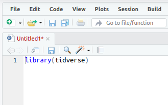
Type or paste the following text at the top of the newly opened R script in the top left panel.

library(tidyverse)

When you’ve put that in, the script title will go red, showing it can now be saved (it should look something like the image below).

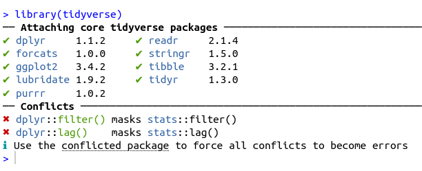
Save the script either with the CTRL + S shortcut, or file > save. Give it whatever name you like, but note that it saves into your self-contained project folder.

Task: Run the library(tidyverse) line

Now we need to actually run that line of code… we can do this in a couple of ways:

In your R script, if no code text is highlighted/selected RStudio will Run the code line by line (or chunk by chunk - we’ll cover that in the taster session).
If a block of text is highlighted, the whole block will run. So e.g. if you select-all in a script and then run it, the entire script will run.

Let’s do #1: Run the code line by line.

To test this, we’ll load the tidyverse library with the code we just pasted in (which is just one line of code at the moment!) Put the cursor at the end of the libary(tidyverse) line in the script (if it’s not there already), either with the mouse or keyboard. (Keyboard navigation is mostly the same as any other text editor like Word, but here’s a full shortcut list if useful.)
Once there, either use the ‘run’ button, top right of the script window, or (much easier if you’re doing this repeatedly) press CTRL+ENTER to run it.

If all is well, you should see the text below in the console - the tidyverse library is now loaded. Huzzah!

Finally - some economic data! Phew.

Well nearly…

Just one more thing first before actual economic data, sorry. We’re just going to load some functions (and install a couple of libraries) that we’ll need.

If of interest, code for these functions are on the github site here.

Task: In the R script, stick this code below the library(tidyverse) line and run it with CTRL+ENTER or the run command

As this will install a couple of libraries for the first time it’ll take about a minute to run.

Note: comments in R begin with a #hash.

#Load some functions and two libraries (and install those libraries if they're not already present)
source('https://bit.ly/rtasterfunctions')

Now we can load some regional GVA data!

Tasks: Load in regional economic data, then look at it in RStudio.

This line takes a comma-separated variable (CSV) file from the web and names it / assigns it to df. Paste it into your script (below the other code we’ve added) and run it.

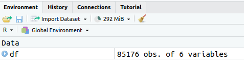
If you look at the environment pane, top right. df should now be there (as in the pic below). Click anywhere on that line in the environment pane - it’ll open a new tab in RStudio with a view of the data attached to df.

# LOAD ITL3 GVA DATA----

#ITL3 zones, SIC sections, current prices, 2023 latest data (minus imputed rent)
df = read_csv('https://bit.ly/rtasteritl3noir')

#This one has imputed rent included if you want it
# df = read_csv('https://bit.ly/rtasteritl3')

What data have we got here?

This is from the latest ONS “Regional gross value added (balanced) by industry: all International Territorial Level (ITL) regions” (The Excel file is available here). Released April 2025, it’s got data up to 2023. It has:

GVA values from 1998 to 2023, broken down by:
ITL3 zones i.e. local authorities rather than MCAs
SIC sections: 18 broad sector categories (max in this data is 45 categories)

Plus…

This is current price data: what the pound value of GVA was in each separate year, unadjusted for inflation
This data can be summed, unlike the inflation-adjusted (chained volume) data (where each sector in each place is inflation-adjusted separately, so can’t be summed)
Because it can be summed, this current price data is great for digging into structural change (e.g. “How have sector proportions changed over time?”) But not so good for real growth analysis.

Let’s start looking at the data in R…

Getting the regional GVA data you want

Today we’re looking at just one example pulled from the Excel sheet. If you want any of the other ready-made CSVs, I’ve pipelined them all to this webpage for the 2025 data.

If you want code for doing any of those extractions, it’s here.

Note: I haven’t yet linked it to jobs data for this year, though that page has it linked for 2022 data.

Task: look at what SIC sector categories are in the data

We can do this by pulling out the unique values from a column.

In R, there are different ways to refer to columns. Here’s a key one: use the object’s name, then a dollar sign. R will then let you autocomplete the column name.

unique(df$SIC07_description)

 [1] "Agriculture, forestry and fishing; mining and quarrying"
 [2] "Manufacturing"                                          
 [3] "Electricity, gas, water; sewerage and waste management" 
 [4] "Construction"                                           
 [5] "Wholesale and retail trade; repair of motor vehicles"   
 [6] "Transportation and storage"                             
 [7] "Accommodation and food service activities"              
 [8] "Information and communication"                          
 [9] "Financial and insurance activities"                     
[10] "Real estate activities, excluding imputed rental"       
[11] "Professional, scientific and technical activities"      
[12] "Administrative and support service activities"          
[13] "Public administration and defence"                      
[14] "Education"                                              
[15] "Human health and social work activities"                
[16] "Arts, entertainment and recreation"                     
[17] "Other service activities"                               
[18] "Activities of households"

Task: do the same for place names

We can use the same method to get the full list of ITL3 place names too (though we’ll use an easier method to pick them out later). Here, we also stick them into alphabetical order.

unique(df$Region_name)[order(unique(df$Region_name))]

“R is brilliant” exhibit A: we can use it to automate/repeat tedious things.

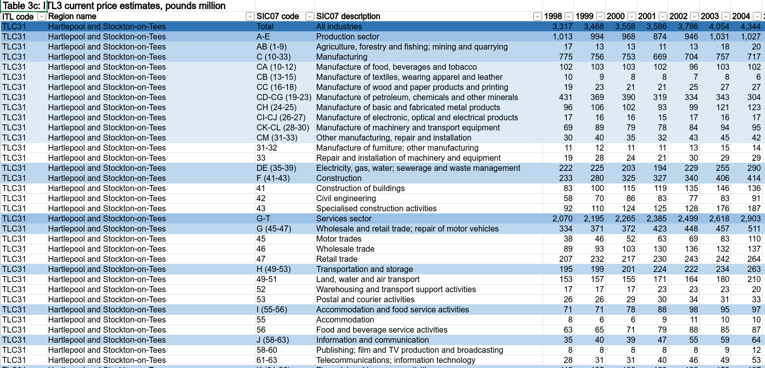
Here’s a sample of what the data looks like in the original Excel file. Different SIC sector levels are nested, there’s one column per year (in R, we’ve made year a single ‘tidy’ column)

The data we’ve attached to the df object comes from that ONS Excel sheet
I’ve used R to get it directly from the web and then extract each CSV separately that might be needed
Each of those nested sector groups gets separated out: goods/services, sections, the full SIC list (45 sectors in this data)
The code for that is here and we run through another example later.
(Is this an example of R code that could be useful to run in powerBI to wrangle data for use?)

Wrangling the data

So - we have our sector/region GVA data in R now - but how to wrangle it by place and sector, to start getting useful info out of it?
Here’s an example of using the tidyverse to do this - we’ll group by sector for the latest year to see its median and range

Task: Wrangle the data to get some summary numbers

We’ll talk about what’s going on here a bit more in the next slide. For now - copy and run the code.

Note: RStudio will run the whole block if press CTRL + ENTER with cursor anywhere in it.

df %>% 
  filter(year == max(year)) %>% 
  group_by(SIC07_description) %>% 
  summarise(
    median_gva = median(value),
    min_gva = min(value),
    max_gva = max(value)
    ) %>% 
  arrange(-median_gva)

# A tibble: 18 × 4
   SIC07_description                                  median_gva min_gva max_gva
   <chr>                                                   <dbl>   <dbl>   <dbl>
 1 Wholesale and retail trade; repair of motor vehic…      998.      113   11342
 2 Manufacturing                                           968       112    4833
 3 Human health and social work activities                 944        87    4412
 4 Construction                                            705       100    3712
 5 Education                                               612.       75    4336
 6 Professional, scientific and technical activities       516.       24   34316
 7 Public administration and defence                       494.       93    7834
 8 Administrative and support service activities           446.       27   12461
 9 Transportation and storage                              350.       38    2283
10 Real estate activities, excluding imputed rental        320.        8    7529
11 Information and communication                           265        13   25073
12 Accommodation and food service activities               264        61    5393
13 Financial and insurance activities                      246         5   74615
14 Electricity, gas, water; sewerage and waste manag…      226        10    2547
15 Other service activities                                157        19    2500
16 Arts, entertainment and recreation                      104.       11    3201
17 Agriculture, forestry and fishing; mining and qua…       43.5       0    1862
18 Activities of households                                  8         2      65

Piping interlude!

That last block of code was piping output of one function into the input of the next, chaining them together. This is super-powerful and useful.

Here’s the principle with a silly toy example using two functions. Dead simple here, but with larger processing chains it quickly becomes indispensible. It’ll crop up a lot as we go.¹

Task: compare standard R function to ‘piping in’ the argument

If typing these out, the keyboard shortcut in RStudio for the pipe operator is CTRL + SHIFT + M.

#Boooo, nested brackets...
sqrt(log10(10000))

[1] 2

#Wooo! Lovely piped functions!
10000 %>% sqrt %>% log10

[1] 2

Getting sector proportions and location quotients

Now we’ll wrangle the data using a function we loaded earlier Blue Peter style (may be showing age there!)
This function adds in columns for what proportion of each place’s economy each sector makes up and, using that, what the location quotient (LQ) is for each sector in each place.

Location quotient (LQ)

In case the LQ is new to anyone: it’s just the proportion of a sector in a place, over its proportion nationally.
So it’s less than one if a sector is less concentrated in a place than the UK average / more than 1 if higher (and 0.5 and 2 if it’s half or double the UK concentration).
This ONS LQ excel sheet has a really clear explanation in the notes.
I’ve made a page on other ways to use the LQ in R here, if of interest.

Task: run this function and glimpse the result in the console.

We stick four arguments into the function - including the data itself, which here we filter to the latest year.

It’s then piped to glimpse, which lets us look at all columns at once by sticking them on their side in the console (a nice way to check our results look sane).

# LOCATION QUOTIENTS/PROPORTIONS----

add_location_quotient_and_proportions(
  df %>% filter(year == max(year)),
  regionvar = Region_name,
  lq_var = SIC07_description,
  valuevar = value
) %>% glimpse

Rows: 3,276
Columns: 13
$ ITL_code                   <chr> "TLC31", "TLC31", "TLC31", "TLC31", "TLC31"…
$ Region_name                <chr> "Hartlepool and Stockton-on-Tees", "Hartlep…
$ SIC07_code                 <chr> "AB (1-9)", "C (10-33)", "DE (35-39)", "F (…
$ SIC07_description          <chr> "Agriculture, forestry and fishing; mining …
$ year                       <dbl> 2023, 2023, 2023, 2023, 2023, 2023, 2023, 2…
$ value                      <dbl> 19, 933, 266, 716, 891, 234, 178, 195, 558,…
$ region_totalsize           <dbl> 7091, 7091, 7091, 7091, 7091, 7091, 7091, 7…
$ sector_regional_proportion <dbl> 0.002679453, 0.131575236, 0.037512340, 0.10…
$ total_sectorsize           <dbl> 20156, 225096, 63700, 154147, 243916, 83906…
$ totalsize                  <dbl> 2200006, 2200006, 2200006, 2200006, 2200006…
$ sector_total_proportion    <dbl> 0.0091617932, 0.1023160846, 0.0289544665, 0…
$ LQ                         <dbl> 0.2924594, 1.2859682, 1.2955631, 1.4411007,…
$ LQ_log                     <dbl> -1.22942932, 0.25151194, 0.25894546, 0.3654…

Tip

Once the code from the next slide is in RStudio, if you CTRL + mouse click on the function name, it’ll take you to the code (if you loaded them above). You’ll see it’s a not-too-elaborate piping operation of the type we were just looking at.

The power of functions is in packaging this kind of ‘need often’ task into flexible, reusable form.

In the next code block we’re running the same code but doing four extra things that we chain together:

We group_split the data into years (one separate dataframe per year)
map each year bundle into the add_location_quotient_and_proportions function
bind_rows it all back together
We also overwrite df with the result (first line) so we’ve kept it (rather than, in the last example, just outputting to the console).

Task: find LQs and proportions for each year and keep the result

Once run, we can also look at the result again via the environment panel.

(Note: you’ll probably get a warning - this is due to a single negative GVA value, it won’t affect anything here.)

While we’re here: highlight just this bit of code: df %>% group_split(year) and then run. We can see what just that chunk is doing exactly what the function name suggests.

#Finding location quotients for each year in the data 
#And then overwriting the df variable with the result
df = df %>%
  group_split(year) %>%
  map(add_location_quotient_and_proportions,
      regionvar = Region_name,
      lq_var = SIC07_description,
      valuevar = value) %>% 
  bind_rows()

Now let’s do something with result:

Pick out one place or local authority: you’ll only need some of the place name you want - here I’m using rotherh to find Rotherham.
For the latest year in the data, pull out the location quotient and sector proportion for that place. And then order, highest to lowest.

Task:

#View a single place...
df %>% filter(
  qg('rotherh',Region_name),
  year == max(year)#get latest year in data
) %>% 
  mutate(regional_percent = sector_regional_proportion *100) %>% 
  select(SIC07_description,regional_percent, LQ) %>% 
  arrange(-LQ)

Output from that code…

Rotherham’s largest sector specialism (highest LQ) is manufacturing for the latest year (and nearly 19% of its economy).

# A tibble: 18 × 3
   SIC07_description                                     regional_percent     LQ
   <chr>                                                            <dbl>  <dbl>
 1 Manufacturing                                                   18.8   1.84  
 2 Construction                                                    12.7   1.81  
 3 Activities of households                                         0.139 1.40  
 4 Transportation and storage                                       5.28  1.38  
 5 Human health and social work activities                         12.8   1.38  
 6 Electricity, gas, water; sewerage and waste manageme…            3.89  1.34  
 7 Public administration and defence                                6.74  1.21  
 8 Wholesale and retail trade; repair of motor vehicles            13.2   1.19  
 9 Administrative and support service activities                    6.47  1.10  
10 Education                                                        7.24  1.05  
11 Accommodation and food service activities                        3.25  1.03  
12 Agriculture, forestry and fishing; mining and quarry…            0.694 0.758 
13 Other service activities                                         1.33  0.733 
14 Arts, entertainment and recreation                               0.774 0.502 
15 Professional, scientific and technical activities                3.09  0.333 
16 Information and communication                                    2.20  0.333 
17 Financial and insurance activities                               1.21  0.123 
18 Real estate activities, excluding imputed rental                 0.159 0.0398

Cheatsheets!

There are a bunch of excellent cheat sheet documents available for many of R’s features. You can easily access them via RStudio’s help menu.

The data tranformation with dplyr sheet covers a lot of the functions we’re using in piping operations.

There’s also an excellent ggplot cheatsheet, among many others. We’ll come back to this one…

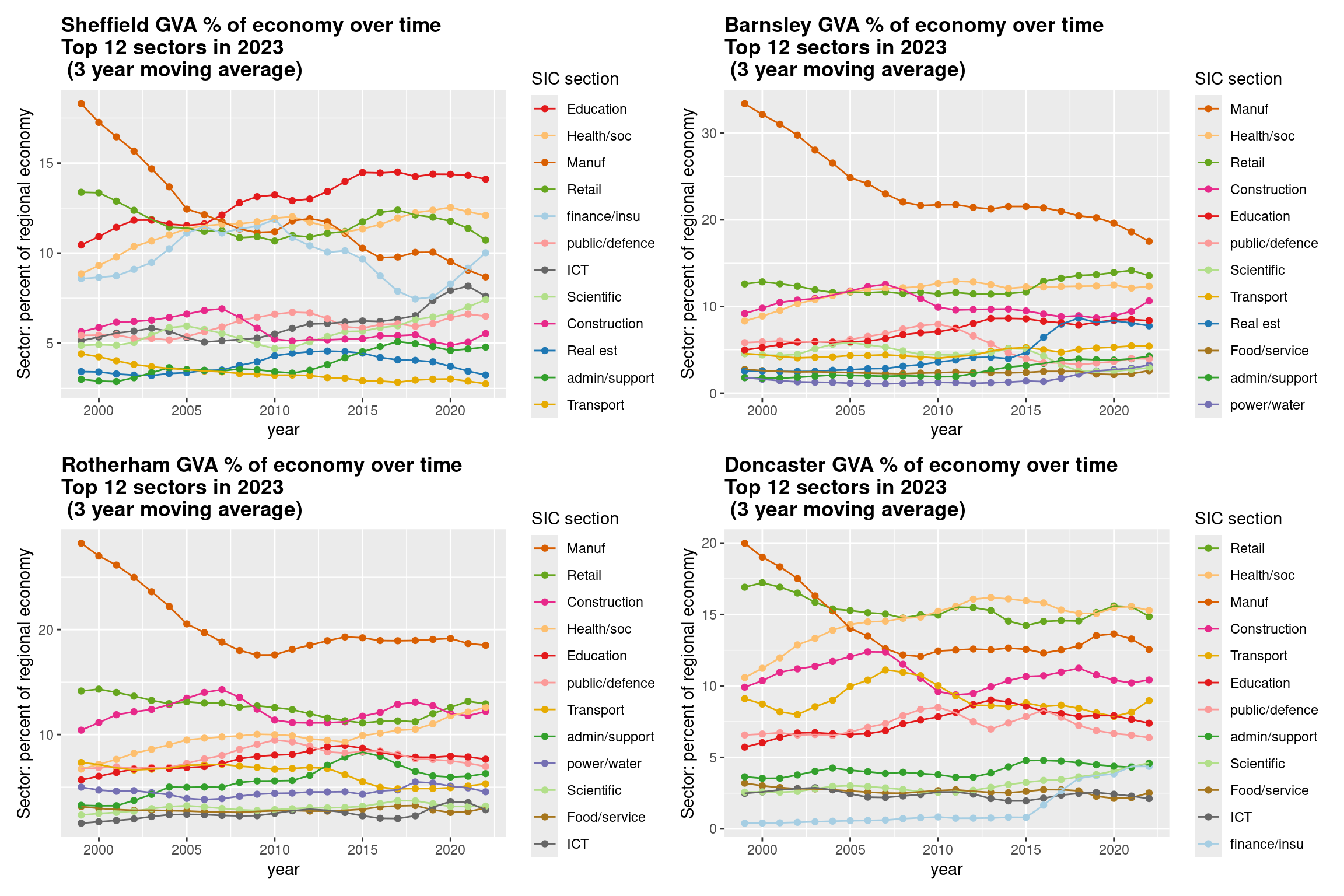
Visualising: how has the structure of places’ economies changed over time?

Let’s plot some of the data. We’ll look at how an ITL3 zone’s broad sectors have changed their proportion over time, to see how those economies have changed structurally.

We’ll do this in 3 stages:

Add in a moving average to smooth the data a little
Pick out the top 12 broad sectors in the latest year
Plot!

Task: apply the moving average to our df data object and pick out the placename we want

You can look at the available ITL3 zones at geoportal.statistics.gov.uk here, if useful for checking names. (Opens in new tab.)

# PLOT STRUCTURAL CHANGE OVER TIME IN ITL3 ZONE----

#Processing before plot

#1. Set window for rolling average: 3 years
smoothband = 3

#2. Make new column with rolling average in (applying to all places and sectors)
#Years are already in the right order, so will roll apply across those correctly
df = df %>% 
  group_by(Region_name,SIC07_description) %>% 
  mutate(
    sector_regional_prop_movingav = rollapply(
      sector_regional_proportion,smoothband,mean,align='center',fill=NA
      )
  ) %>% 
  ungroup()

#3. Pick out the name of the place / ITl3 zone to look at
#We only need a bit of the name...
place = getdistinct('doncas',df$Region_name)

#Check we found the single place we wanted (some search terms will pick up none or more than one)
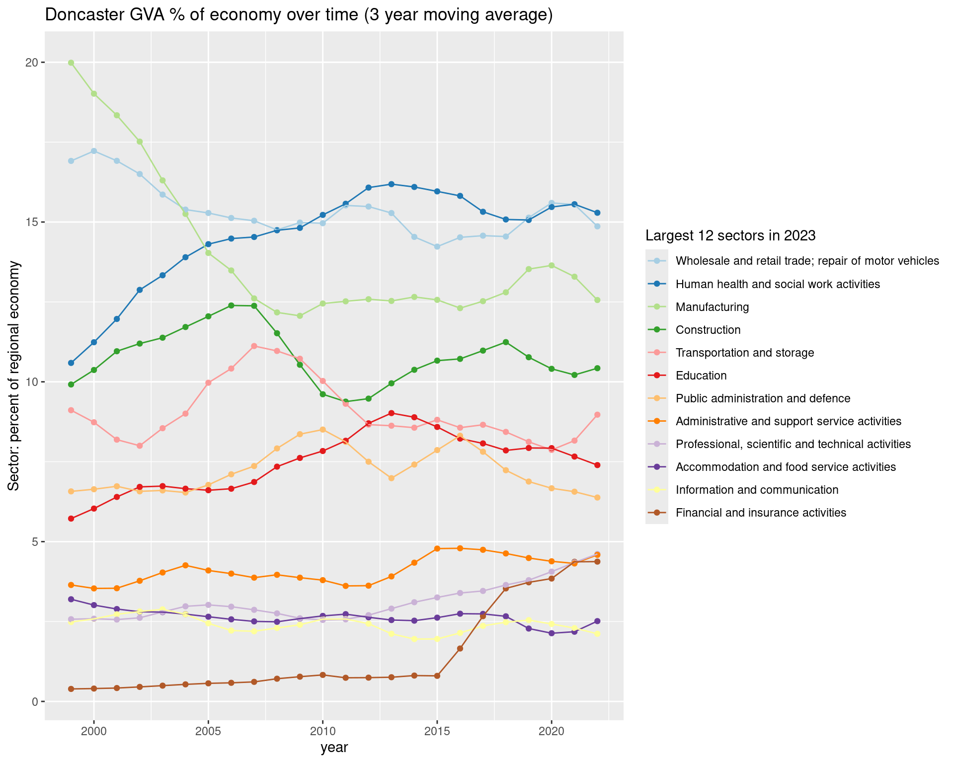
place

[1] "Doncaster"

Task: for our chosen place, pick out the largest proportion sectors in the most recent year

Here, we filter to get our place and year, arrange in reverse order of moving average, slice off the top 12 and pull out the sector names.

# top 12 sectors in latest year
top12sectors = df %>%
  filter(
    Region_name == place,
    year == max(year) - 1#to get 3 year moving average value
  ) %>%
  arrange(-sector_regional_prop_movingav) %>%
  slice_head(n= 12) %>%
  select(SIC07_description) %>%
  pull()

GGPLOT interlude!

In the next slide, we finally make an actual chart. Phew.
There’s a lot going on in ggplot, the package we’ll be using to visualise data - but it’s worth mentioning that its principles are actually clear and consistent.
You’ll see it has an aes argument - that’s short for aesthetics. An aesthetic is any single distinct plot element - like the x or y axis, colour, shape, size etc.

The rule is simple: you map one data column to one aesthetic. This is another tidy data principle, and its the reason we have years in their own column, so year can be mapped to one axis.
We’ll see later with geographical zones - categorical variables also get mapped to single aesthetics.
The ggplot cheatsheet shows, for all plot types, what aesthetics are available.

Task: plot smoothed sector proportion over time using ggplot

#Plot! 
ggplot(df %>%
         filter(
           Region_name == place,
           SIC07_description %in% top12sectors,
           !is.na(sector_regional_prop_movingav)#Remove NAs created by 3 year moving average
           ),
       aes(x = year, y = sector_regional_prop_movingav * 100, colour =
             fct_reorder(SIC07_description,-sector_regional_prop_movingav) )) +
  geom_point() +
  geom_line() +
  scale_color_brewer(palette = 'Paired', direction = 1) +
  ylab('Sector: percent of regional economy') +
  labs(colour = paste0('Largest 12 sectors in ',max(df$year))) +
  ggtitle(paste0(place, ' GVA % of economy over time (', smoothband,' year moving average)'))

Resulting plot is on on next slide –>

Before moving on…

There are a load more examples of using this data for comparing places, doing location quotients etc at my regional econ tools website (of course produced using R!)
This intro has basic examples, this digs more into using LQs to put places in national context, this looks at ways to see how GVA ‘gaps’ between places change over time.

Real GVA growth over time

Current prices are great and everything - loads of value being able to examine relative change, and things actually adding up. But they’re not real prices¹, so can’t be used to understand real growth over time.

For this, we have to use chained volume data that adjusts for inflation…

So next we load data for the same sectors and ITL3 zones, but it’s chained volume GVA figures, inflation-adjusted to 2022 money value.

We’ll then pick out a single place to examine. You can use a small part of a local authority / place name to return the full name that we’ll use to filter the data.

We’ll check it’s returned what you want though. For example, glouc will return a couple of different places with ‘Gloucester’ in.

Tasks: Load in the chained volume data for ITL3 zones and SIC sections, then pick a place name to examine

# CHAINED VOLUME ITL3 DATA----

df.cv = read_csv('https://bit.ly/rtasteritl3cvnoir')

#Get the text for an ITL3 zone by searching for a bit of the name
place = getdistinct('barns',df$Region_name)

#Check we got just one place!
place

[1] "Barnsley"

#If needed, code to list all ITL3 place names again
#unique(df.cv$Region_name)

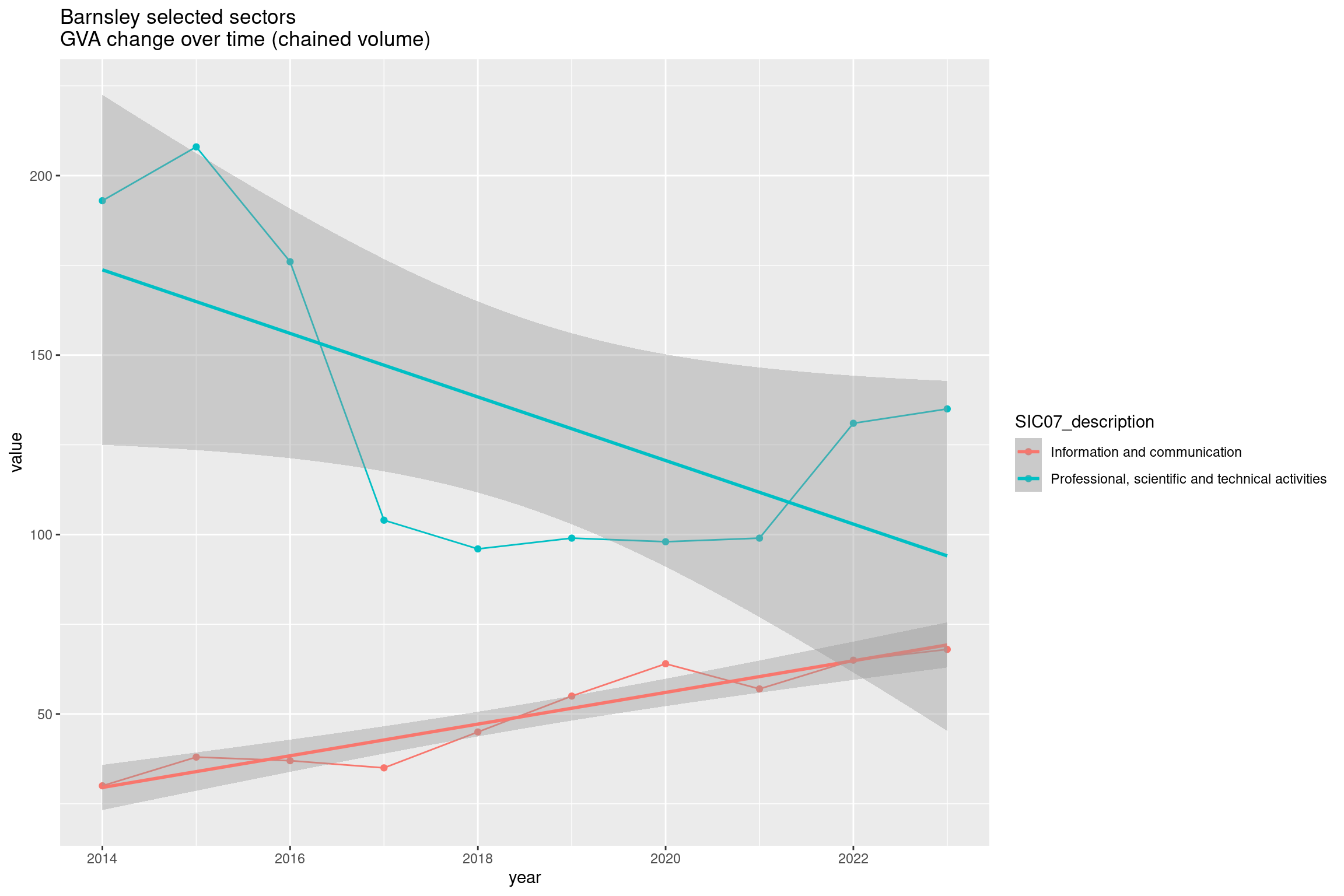
Now we’ll examine sector growth trends, looking at average growth over time. To start with, let’s pick out a couple of sectors for our chosen place.

Task: Plot trends over time for a couple of sectors using ggplot.

Set a start/end year (here, the most recent decade). Note: two sector names are searched for here, separating with a | vertical bar meaning or. Reminder: you can look at the full list of available sectors with unique(df.cv$SIC07_description)

startyear = 2014
endyear = 2023

#Pick out single slopes to illustrate
ggplot(
  df.cv %>% filter(
    year %in% startyear:endyear,
    Region_name == place,
    qg('information|professional', SIC07_description)
  ),
  aes(x = year, y = value, colour = SIC07_description)
) +
  geom_point() +
  geom_line() +
  geom_smooth(method = 'lm') +
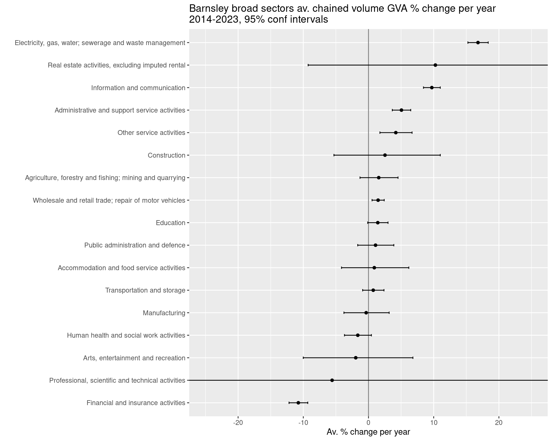
  ggtitle(paste0(place, ' selected sectors\nGVA change over time (chained volume)'))

Next, we’re going to find linear trends for every sector in our chosen place and compare them, including some confidence intervals. To do this we’ll:

Use another pre-made function loaded earlier that finds linear slopes and standard errors for each group (each sector in this case), using log values so change is comparable.
Do a bit of wrangling and then plot average % change per year for each sector.

Task: Get slopes and confidence intervals for each sector in our chosen place

The function has a ‘use Newey West estimators’ option - better standard errors for sticking lines through time series data (open contibutions to improve trend analysis here would be very welcome!)

#Get all slopes for sectors in that place
slopes = get_slope_and_se_safely(
  df.cv %>% filter(
    year %in% startyear:endyear,
    Region_name == place,
    !qg('households', SIC07_description)
    ), 
  SIC07_description, 
  y = log(value), 
  x = year, 
  neweywest = T)


#Add 95% confidence intervals around the slope
slopes = slopes %>% 
  mutate(
    ci95min = slope - (se * 1.96),
    ci95max = slope + (se * 1.96)
  )

Task:

#Adjust to get percentage change per year
slopes = slopes %>% 
  mutate(across(c(slope,ci95min,ci95max), ~(exp(.) - 1) * 100, .names = '{.col}_percentperyear'))

#Plot the slope with those confidence intervals
ggplot(slopes, aes(x = slope_percentperyear, y = fct_reorder(SIC07_description,slope))) +
  geom_point() +
  geom_errorbar(aes(xmin = ci95min_percentperyear, xmax = ci95max_percentperyear), width = 0.1) +
  geom_vline(xintercept = 0, colour = 'black', alpha = 0.5) +
  coord_cartesian(xlim = c(-25,25)) +
  xlab('Av. % change per year') +
  ylab("") +
  ggtitle(paste0(place, ' broad sectors av. chained volume GVA % change per year\n',startyear,'-',endyear,', 95% conf intervals'))

Plot in next slide –>

More growth analysis: ITL2 zones

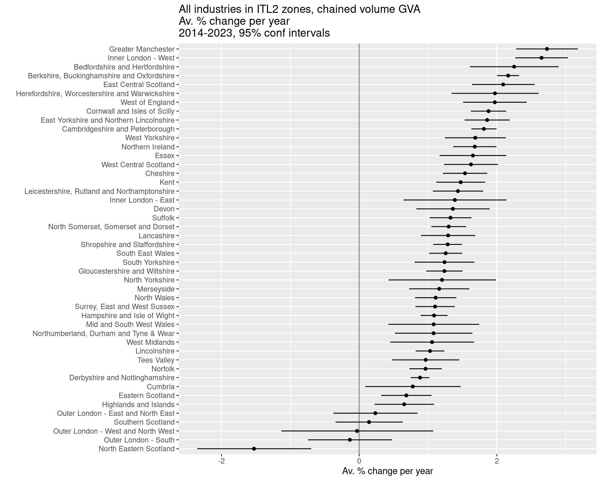
Let’s actually run through extracting data from an online Excel sheet. It’s not too much work. We’ll use it to look at growth rates for the entire economies of mayoral authorities and other ITL2 zones.

We use the readxl package - this is already installed in posit.cloud RStudio. If you’re working in RStudio on your own machine, here’s some code to check if you have it installed and install it if not.

Task: Check if readxl is installed and install if not

# EXAMPLE OF GETTING DATA DIRECTLY (GET NATIONAL SIC SECTION DATA)----

#Check readxl is already installed, install if not.
if(!require(readxl)){
  install.packages("readxl")
  library(readxl)
}

Then onto getting the data directly and processing it…

Task: Copy and run this code to get data directly from the ONS regional/industry GVA Excel file

We download a temporary local copy and then extract from a sheet and cell range we define using the readxl package.

#2025:
url1 <- 'https://www.ons.gov.uk/file?uri=/economy/grossvalueaddedgva/datasets/nominalandrealregionalgrossvalueaddedbalancedbyindustry/current/regionalgrossvalueaddedbalancedbyindustryandallinternationalterritoriallevelsitlregions.xlsx'
p1f <- tempfile(fileext=".xlsx")
download.file(url1, p1f, mode="wb") 

itl2.all <- read_excel(path = p1f,range = "Table 2a!A2:AD4556")

names(itl2.all) <- gsub(x = names(itl2.all), pattern = ' ', replacement = '_')

itl2.all = itl2.all %>% 
  filter(SIC07_description == 'All industries') %>% 
  pivot_longer(`1998`:names(itl2.all)[length(names(itl2.all))], names_to = 'year', values_to = 'value') %>% #get most recent year
  mutate(year = as.numeric(year))

Now we have the data in the itl.all object in the form we want, we’ll do as we did above for sectors in one place - find linear slopes for each ITL2 zone and some confidence intervals.

Task: choose a time window and find OLS slopes for each ITL2 zone

startyear = 2011
endyear = 2023

#Get all slopes for sectors in that place
slopes = get_slope_and_se_safely(
  itl2.all %>% filter(year %in% c(startyear:endyear)), 
  Region_name,
  y = log(value), 
  x = year, 
  neweywest = T)


#Add 95% confidence intervals around the slope
slopes = slopes %>% 
  mutate(
    ci95min = slope - (se * 1.96),
    ci95max = slope + (se * 1.96)
  )

Finally, we plot the slopes to show average percent change over time…

Task: plot each ITL2’s linear slopes with confidence intervals

#Adjust to get percentage change per year from log slopes
slopes = slopes %>% 
  mutate(across(c(slope,ci95min,ci95max), ~(exp(.) - 1) * 100, .names = '{.col}_percentperyear'))

#Plot the slope with those confidence intervals
ggplot(slopes, aes(x = slope_percentperyear, y = fct_reorder(Region_name,slope))) +
  geom_point() +
  geom_errorbar(aes(xmin = ci95min_percentperyear, xmax = ci95max_percentperyear), width = 0.1) +
  geom_vline(xintercept = 0, colour = 'black', alpha = 0.5) +
  xlab('Av. % change per year') +
  ylab("") +
  ggtitle('All industries in ITL2 zones, chained volume GVA\nAv. % change per year\n2014-2023, 95% conf intervals')

Things we haven’t covered

Building full pipelines from the data wrangling above can include:
- Preparing reports in R. Here’s an example looking at business dynamism using ONS data.
- Using github to complete the pipeline by presenting online (e.g. these slides!)
- Interactives in R e.g. Companies House ‘most common sector’ hexmap; interactive employment report.
- Making dashboards using R Shiny e.g. South Yorkshire Companies House employee change dashboard.

Other things we could cover another time (links to examples)

Directly accessing NOMIS data in R and harmonising with other sources. Examples: BRES jobs. Good GVA demoninators like 16-64s or 16+, per filled job, pop count, per hour worked (example of plotting GVA over each of these). SICSOC industry vs occupation (dashboard example in SICSOC tab here).
Harmonised regional GVA and jobs data. I’ve done that here but the GVA/jobs link needs a 2023 update.

Next?

Would any of the above be of interest for future R sessions?
Is there anything I’ve not mentioned that would be good?
Happy to chat - d dot olner at sheffield dot ac dot uk or message me on LinkedIn.

BONUS MATERIAL

Multiple proportion plots with consistent sector colours

Task:

n <- length(unique(df$SIC07_description))
set.seed(12)
qual_col_pals = RColorBrewer::brewer.pal.info[RColorBrewer::brewer.pal.info$category == 'qual',]
col_vector = unlist(mapply(RColorBrewer::brewer.pal, qual_col_pals$maxcolors, rownames(qual_col_pals)))

randomcols <- col_vector[10:(10+(n-1))]

#Do once!
getplot <- function(place){
  
  df = df %>% 
    filter(!qg("Activities of households|agri",SIC07_description)) %>% 
    mutate(
      SIC07_description = case_when(
        grepl('defence',SIC07_description,ignore.case = T) ~ 'public/defence',
        grepl('support',SIC07_description,ignore.case = T) ~ 'admin/support',
        grepl('financ',SIC07_description,ignore.case = T) ~ 'finance/insu',
        grepl('agri',SIC07_description,ignore.case = T) ~ 'Agri/mining',
        grepl('electr',SIC07_description,ignore.case = T) ~ 'power/water',
        grepl('information',SIC07_description,ignore.case = T) ~ 'ICT',
        grepl('manuf',SIC07_description,ignore.case = T) ~ 'Manuf',
        grepl('other',SIC07_description,ignore.case = T) ~ 'other',
        grepl('scientific',SIC07_description,ignore.case = T) ~ 'Scientific',
        grepl('real estate',SIC07_description,ignore.case = T) ~ 'Real est',
        grepl('transport',SIC07_description,ignore.case = T) ~ 'Transport',
        grepl('entertainment',SIC07_description,ignore.case = T) ~ 'Entertainment',
        grepl('human health',SIC07_description,ignore.case = T) ~ 'Health/soc',
        grepl('food service activities',SIC07_description,ignore.case = T) ~ 'Food/service',
        grepl('wholesale',SIC07_description,ignore.case = T) ~ 'Retail',
        .default = SIC07_description
      )
    )
  
  top12sectors = df %>%
    filter(
      Region_name == place,
      year == max(year) - 1#to get 3 year moving average value
    ) %>%
    arrange(-sector_regional_prop_movingav) %>%
    slice_head(n= 12) %>%
    select(SIC07_description) %>%
    pull()
  
  
  ggplot(df %>% 
           filter(
             Region_name == place, 
             SIC07_description %in% top12sectors,
             !is.na(sector_regional_prop_movingav)#Remove NAs created by 3 year moving average
           ), 
         aes(x = year, y = sector_regional_prop_movingav * 100, colour = fct_reorder(SIC07_description,-sector_regional_prop_movingav) )) +
    geom_point() +
    geom_line() +
    scale_color_manual(values = setNames(randomcols,unique(df$SIC07_description))) +#set manual pastel colours matching sector name
    ylab('Sector: percent of regional economy') +
    theme(plot.title = element_text(face = 'bold')) +
    labs(colour = 'SIC section') +
    # scale_y_log10() +
    ggtitle(paste0(place, ' GVA % of economy over time\nTop 12 sectors in ',max(df$year),'\n (', smoothband,' year moving average)'))
  
  
}

places = getdistinct('doncas|roth|barns|sheff',df$Region_name)

plots <- map(places, getplot)

patchwork::wrap_plots(plots)