Demand or supply?
Q4: three signals, three downturns, fifteen industries
In short (15 industries × 3 downturns = 45 cells; rules fixed before the data were seen):
- The three signals agree no more often than chance would give. Fleiss’ kappa is 0.02 and Krippendorff’s alpha 0.07. Raw agreement looks high, but 52 of the 54 decisive labels from firms’ surveys and the labour market say “demand”, so matching is mostly what chance gives. Only 12 of 45 cells get a clear label from all three.
- Where they do agree, it’s demand: 9 cells are demand on all three signals and 15 on two of three. One cell is supply (construction, 2022–23).
- The price–quantity test is weakly identified everywhere. No industry passes the standard strength test (ρ² > 0.5) in any downturn under gross output, so a label says a shock of that kind hit, not which dominated.
- The price index flips half the labels. Using the GVA deflator instead of output prices changes 50% of the labels, and 32% swap between demand and supply.
- One rule decides 2022–23. Firms cited rising costs far more than shortages or weak demand. Whether rising costs count as supply decides the downturn, and they could signal either; that question has its own page.
The question is the plan’s Q4: how can we tell whether output fell because demand fell or because supply did? The method review is R4’s (the methods note); the pilot is A3’s (the pilot note, 2026-11-04), whose rules were written down before any data were downloaded. Scripts: claude_research/productivity/R/a3_run_all.R runs claude_research/productivity/R/a3_01_download.R to claude_research/productivity/R/a3_08_checks.R.
1 The rules, fixed before results
The textbook signature. A demand shock moves price and quantity the same way; a supply shock moves them in opposite directions (Shapiro 2022). Read (RBA 2024) adds a warning: a label carries information only where the price and quantity surprises are strongly correlated.
Three signals, each scored D (demand), S (supply), B (both, firms’ surveys only) or A (ambiguous or no data):
- Prices against quantities. For each industry and quarter, a rolling 10-year VAR in quarterly log changes of output price and volume (4 lags). The surprises are summed over the downturn; a sum within 0.1 standard deviations of zero is ambiguous. Primary lens: gross output prices (producer prices, services producer prices, or CPI components where those don’t exist) against GDP(O) volumes.
- Firms’ stated constraints. The share of firms citing insufficient demand, against those citing shortages of labour, materials or capacity, each compared with its own pre-downturn normal (more than 1 standard deviation above it). Sources: the European Commission’s harmonised business surveys for the UK (collected by the CBI, public to 2020) for 2008–09 and 2020; ONS’s BICS for 2022–23.
- The labour market. Demand if hours or jobs fall and the vacancy rate falls; supply if they fall while vacancies hold or rise and pay growth picks up.
Downturns and industries: 2008 Q2–2009 Q2, 2020 Q2, and 2022 Q1–2023 Q2, for 15 industries from food and drink to legal services. Agreement is scored with Fleiss’ kappa and Krippendorff’s alpha, and every disagreement gets a likely reason, labelled as a judgment.
2 The grid
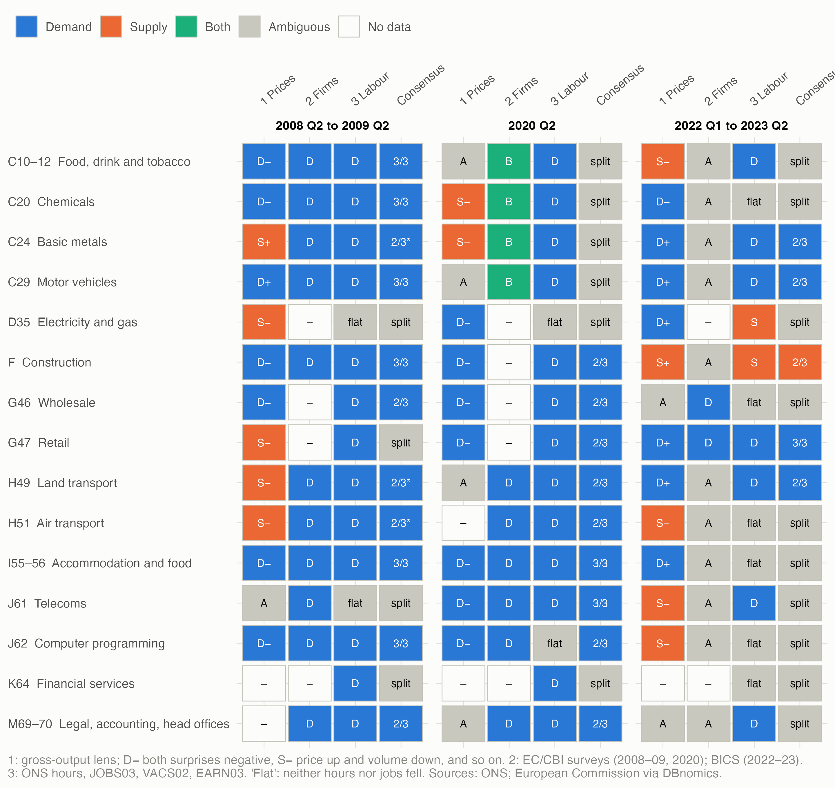
- 2008–09 looks demand-led on the surveys and the labour market: consensus in 11 of 15 industries.
- 2020 is mixed: manufacturers reported material shortages as well as weak demand (“both”).
- 2022–23 is mostly undecided: consensus in only 5 industries. Construction is the one supply cell.
3 Prices against quantities, and the lens
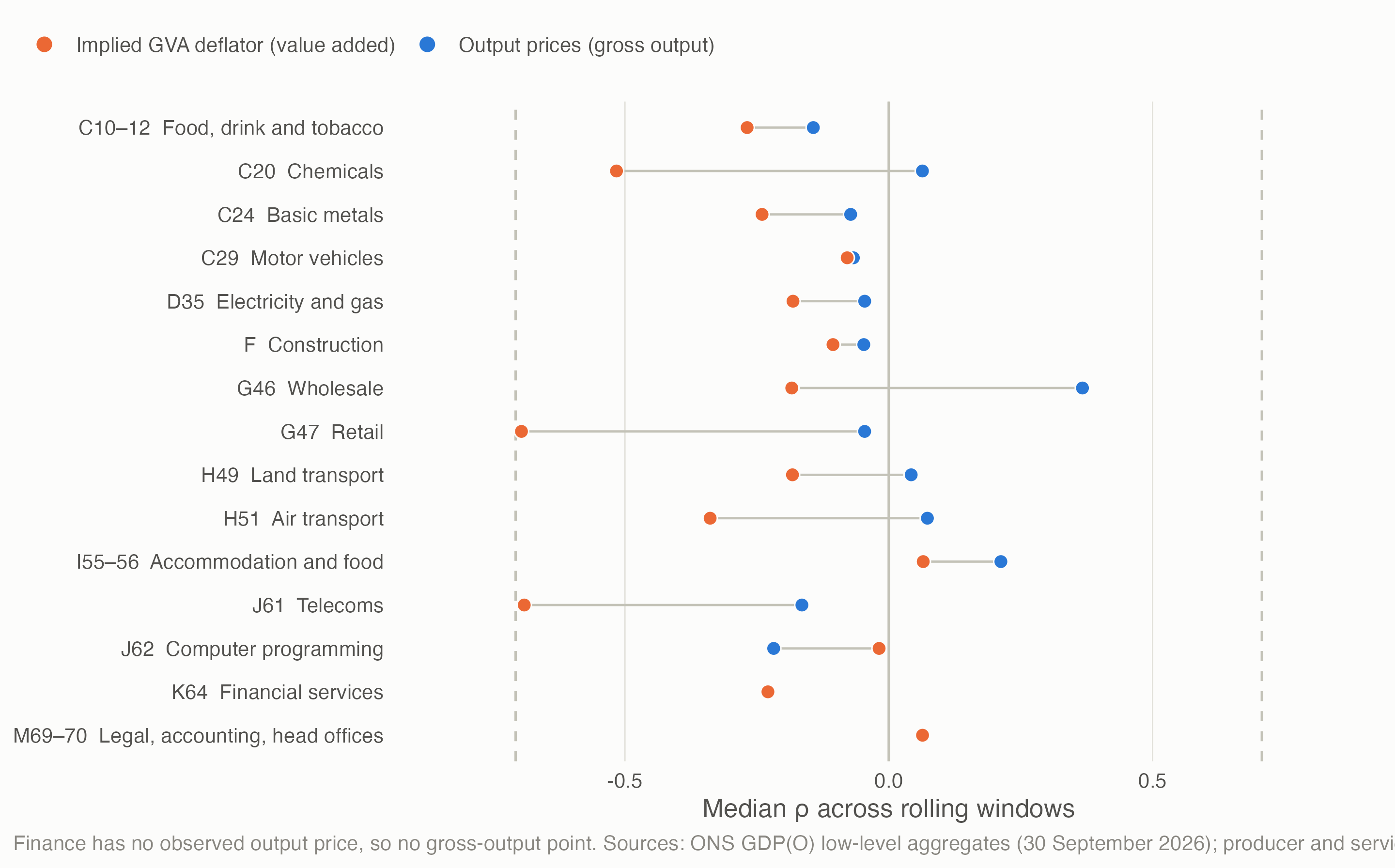
- ρ is small under output prices. Across the scored windows, |ρ| has a median of 0.17, and none reaches ρ² > 0.5. Read’s identified set for supply’s share then covers nearly the whole range: the label can’t say which kind of shock dominated.
- The value-added lens looks better identified, for the wrong reason. Its strongly negative ρ comes where ONS derives price or volume from the other (the implied GVA deflator is current prices ÷ chained volume), so any error moves the two surprises in opposite directions: “division bias”, as R4 predicted. It biases labels towards supply.
- The lens flips half the labels. Of the 40 cells with data under both lenses, 20 change and 13 switch between demand and supply. Changing only the price index, within the gross-output lens, changed 2 of 9.
- Two predictions from the Q5 frame show up. A margin squeeze: land and air transport in 2008–09 read as supply in output prices (fuel costs pushed prices up as volumes fell) but demand in value added. And sticky prices: in 2020 Q2 several industries’ price surprises were too small to classify while volumes fell, as in the frame’s worked example 4 (page 4).
4 Firms’ stated constraints
| Episode | Sector | Insufficient demand | Labour shortage | Material or equipment shortage | Financial constraints |
|---|---|---|---|---|---|
| 2008–09 | Construction | 54% (z 9.9) | 2% (z −2.5) | 0% (z −1.2) | 17% (z 11.9) |
| 2008–09 | Manufacturing | 79% (z 1.2) | 10% (z −1.4) | 17% (z −1.4) | 9% (z 7.1) |
| 2008–09 | Services | 65% (z 2.6) | 16% (z −2.1) | 1% (z −1.2) | 12% (z −0.2) |
| 2020 | Manufacturing | 75% (z 1.9) | 25% (z 0.5) | 45% (z 3.5) | 33% (z 9.2) |
| 2020 | Services | 71% (z 5.0) | 12% (z −2.8) | 0% (z −1.8) | 57% (z 10.6) |
| Sector | Insufficient domestic demand | Insufficient international demand | Shortage of labour | Shortage of materials | Lack of equipment | Cost of materials | Cost of labour | Financial costs |
|---|---|---|---|---|---|---|---|---|
| Accommodation and food service activities | 16.1 | 2.2 | 16.4 | 4.0 | 3.1 | 52.1 | 38.2 | 28.1 |
| Construction | 6.6 | 0.0 | 13.0 | 11.2 | 1.5 | 44.2 | 22.7 | 11.9 |
| Information and communication | 10.7 | 4.6 | 2.9 | 3.7 | 0.3 | 7.2 | 7.8 | 8.8 |
| Manufacturing | 17.6 | 5.6 | 9.2 | 12.4 | 2.1 | 48.5 | 16.5 | 13.2 |
| Professional, scientific and technical activities | 10.2 | 3.4 | 5.0 | 3.1 | 0.7 | 10.4 | 9.6 | 8.8 |
| Transportation and storage | 8.1 | 2.3 | 14.7 | 6.9 | 1.6 | 21.0 | 15.5 | 18.1 |
| Wholesale and retail trade; repair of motor vehicles and motorcycles | 18.2 | 4.4 | 7.2 | 7.9 | 1.0 | 35.4 | 13.4 | 17.7 |
- 2008–09 was a demand shock in every surveyed sector: demand shares well above normal, labour and material shortages below. Counting financial constraints as supply turns manufacturing and construction to “both”: the credit crunch.
- In 2020 manufacturers were short of materials as well as demand; services firms were short of demand.
- In 2022–23 firms cited costs, not shortages or demand. The pre-registered rule counts only shortages as supply, so most sectors come out ambiguous. Counting the costs of labour and materials as supply turns five of seven sectors to supply. Rising costs could signal either, which is why they get their own page.
5 The labour market
- The vacancy rule does almost all the work. The job openings rate fell by more than 10% in 43 of 45 cells, so the label mostly comes down to whether hours or jobs fell. Only energy and construction held their vacancy rates, both in 2022–23, and with pay growth picking up both read as supply.
- “Flat” in 10 cells, where neither hours nor jobs fell.
- 2022–23’s baseline is a vacancy peak. The baseline quarter, 2021 Q4, sits at the post-lockdown record, so a return towards normal reads as weak demand. A 2019 baseline is the obvious test, but it would be a choice made after seeing the results.
6 Agreement
| Pair | Same decisive label, share of all cells | Cells where both decisive | Agree when both decisive |
|---|---|---|---|
| Prices and firms | 22% | 13 | 77% |
| Prices and labour | 38% | 26 | 65% |
| Firms and labour | 36% | 16 | 100% |
| Set | Fleiss’ kappa | Krippendorff’s alpha |
|---|---|---|
| As pre-registered | 0.02 | 0.07 |
| Signal 1 value added instead | 0.06 | 0.06 |
| Signal 2 with finance as supply | −0.07 | −0.15 |
| Primary, episode 2008-09 | 0.11 | −0.10 |
| Primary, episode 2020 | −0.16 | 0.05 |
| Primary, episode 2022-23 | −0.06 | 0.20 |
High raw agreement and near-zero kappa go together because one label dominates: when nearly every survey and labour-market label is “demand”, two signals match often by chance, and kappa and alpha measure agreement beyond that.
The disagreements. 9 cells have one signal saying demand and another supply. The likely reasons are judgments made after seeing the results:
| Cell | Labels (1 / 2 / 3) | Likely reason (a judgment) |
|---|---|---|
| C10–12 Food, drink and tobacco, 2022–23 | S− / A / D | Mixed shock: input costs passed into prices as volume fell; firms cited costs, not shortages or demand |
| C20 Chemicals, 2020 | S− / B / D | Mixed shock: firms reported both weak demand and material shortages |
| C24 Basic metals, 2008–09 | S+ / D / D | Phases inside the window: the trough quarter reads demand, but 2009’s volume rebound against falling prices dominates the sum |
| C24 Basic metals, 2020 | S− / B / D | Mixed shock, as for chemicals |
| D35 Electricity and gas, 2022–23 | D+ / A / S | Measurement: volume is physical output, and the volume surprise changes sign between lenses |
| G47 Retail, 2008–09 | S− / A / D | Mixed shock, plus measurement: retail volume is sales deflated by the same price index, so a price error becomes an opposite volume error |
| H49 Land transport, 2008–09 | S− / D / D | Margin squeeze: fuel costs raised prices as volume fell; value added reads demand |
| H51 Air transport, 2008–09 | S− / D / D | Margin squeeze, as for land transport |
| J61 Telecoms, 2022–23 | S− / A / D | Measurement: volume is turnover deflated by the same price index, so price and volume surprises come in opposite pairs almost by construction |
7 What this means
- No single signal can be trusted alone, and the three rarely confirm one another. Report the label with its strength (ρ), its lens, and the other signals beside it.
- Prefer gross-output prices to GVA deflators for the sign test: the value-added lens adds division bias and flips labels through margins.
- Firms’ own reports are the most direct evidence, but they are coarse (broad sectors), and in 2022–23 they mostly say “costs”, which the signs can’t sort without more structure (page 6).
8 Open questions
- Do rising costs count as supply? Decision 14: they could signal either. Page 6 sets out ways to tell them apart.
- Sensitivities chosen after the results (a 2019 vacancy baseline, a wider ambiguous band, shorter windows, a majority-of-quarters rule) would have to be labelled as such.
- More survey data: the Bank of England Agents’ scores, BICS waves before April 2022, or a CBI licence would fill the gaps (energy and finance have no public survey of constraints; construction none in 2020).
- Regions: carrying the national labels to regions by shift-share, and a Brexit episode, are still to do.
- A MONIAC2 deflator slider would show the label flipping with the price index; it should change only the current quarter’s deflator, since a deflator that differs in every quarter also moves the lagged forecasts.
Data and code. A3’s scripts, run by claude_research/productivity/R/a3_run_all.R: downloads (claude_research/productivity/R/a3_01_download.R), series (claude_research/productivity/R/a3_02_series.R), the three signals (claude_research/productivity/R/a3_03_signal1.R, claude_research/productivity/R/a3_04_signal2.R, claude_research/productivity/R/a3_05_signal3.R), scoring (claude_research/productivity/R/a3_06_scoring.R) and checks (claude_research/productivity/R/a3_08_checks.R). Sources: ONS GDP(O) low-level aggregates (30 September 2026), producer and services producer prices (vintages of 21 October 2026, after ONS’s October 2025 correction), CPI (MM23), retail sales deflators, construction output, JOBS03, VACS02, EARN03, output per hour by division (hours); BICS; European Commission business surveys via DBnomics. Full working, including the pre-registered rules and every change the data forced: the pilot note.