The 2D frame and “potential”
Q5: comparing sectors in money, and four meanings of potential
In short:
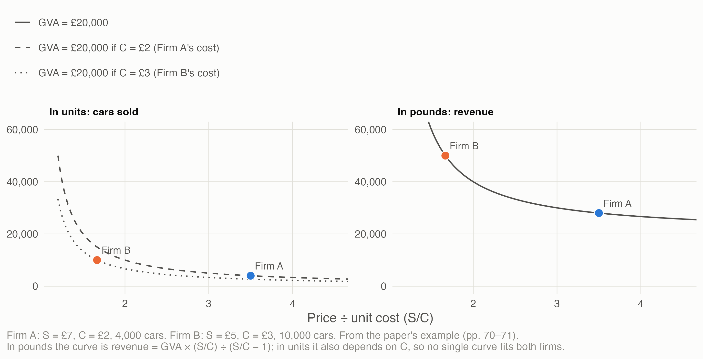
- Webber’s 2D rectangle, GVA = (S − C) × Q, travels across sectors only in money. On the paper’s own axes its two example firms with equal GVA don’t share an isoGVA curve; measured in pounds of sales, they sit exactly on one.
- The unit decides what shrinkflation is. Per bar it’s a productivity gain; per gram it’s inflation. Official statistics read it as inflation in retail, but in food manufacturing it depends on what makers report to ONS.
- “Potential” can mean four things, and each gives a different demand gap for the same industry. Engineering capacity makes every quarter a shortage. Firms’ normal capacity use gives a gap either way. A statistical filter shrinks a long slump towards zero. Surveys measure the sign, not the size.
- Whether potential adapts to demand is the argument in one dial. If firms’ “normal” drifts towards actual output, a long slump turns into lower potential productivity, and the demand shortage disappears from view.
- The UK data show the filter effect. Fitted with only the data available at the time, a standard trend for UK GDP caught down to the post-2008 slump within a few years.
The question is the plan’s Q5: Webber & Huaccha’s 2D model may break comparability across sectors, because it counts goods rather than money; how should it be conceived to widen the idea of productivity? This page draws on the frame (the Q5 frame, 2026-11-03) and R5’s answers to its open points (R5’s note, 2026-11-04), and adds the plots asked for in decision 11. Script: claude_research/productivity/R/c1_potential.R.
1 Where Webber’s 2D model can travel
Webber & Huaccha (2024) draw GVA as a rectangle: the margin per unit (price S less bought-in cost C) times units sold, Q. In the paper, S and Q are a point on one product’s demand curve, and Q is a count of that product’s units. That’s what makes it vivid, and what stops it travelling: a count of cars can’t be compared with a count of haircuts.
So the model has three homes at three scales, kept apart:
| Scale | Unit of Q | Comparable | Use |
|---|---|---|---|
| One product | Its own units | Within the product only | The paper’s demand-curve reading: status goods, shrinkflation, pricing power |
| Across sectors, one year | £ of sales: the rectangle becomes revenue × value-added share | Yes | Comparing sectors and places, as on pages 2 and 3 |
| Over time | £ at reference-year prices | As growth rates, with the deflator named | Linking Webber’s channels to official real GVA |
The unit decides what shrinkflation is. A 200 g bar becomes 180 g at £1; ingredients cost 0.25p a gram; 1,000 bars are sold. Nominal GVA rises 10%.
| Lens | Real output | Real GVA | GVA deflator | Reads as |
|---|---|---|---|---|
| Per bar (the paper’s) | Unchanged | 10% | 0% | A productivity gain: the same bars from less chocolate |
| Per gram (as CPIH treats it) | −10% | −10% | +22.2% | Inflation (11.1% dearer per gram), and less output |
What official statistics do (R5, from ONS’s methods documents):
- Consumer prices (CPI, CPIH) adjust for pack size pro rata. ONS’s own example: an 85 g bar becoming 80 g at the same price is “in effect … paying 6% more”.
- Producer prices treat a change in units of sale as a change of specification, recording only the “pure” price change, but this “generally relies on advice from respondents”. No pro-rata size rule is documented.
- So in retail, whose output ONS deflates with CPI-based Retail Sales Index deflators, shrinkflation reads as inflation. In food and drink manufacturing, deflated with producer prices, it reads as inflation only if the maker reports the change and ONS records a per-unit price rise. If not, the annual double-deflated figures read it as a productivity gain, as the paper claims. The documents don’t say which happens in practice.
Deflation moves a power struggle; it doesn’t hide it. In the paper’s supermarket example the supermarket pays dairies 10p less per litre and cuts its own price by 5p (with a £1.00 price and £0.70 cost, illustratively). The supermarket’s nominal GVA rises 16.7% and the dairy’s falls 16.7%, but real GVA is unchanged for both: the shift goes into their GVA deflators, the price of value added. So anyone reading only real GVA per hour misses it, and regional “real” GVA, built with national industry deflators, keeps part of the transfer. Hence a reporting rule from the frame: wherever real GVA per hour is shown, put the margin price beside it.
2 Four meanings of potential
The paper says “GVA is the sum of potential productivity and demand excess/shortage”. On our reading that’s an output gap, mainly in Q:
\[ \text{GVA} = (S - C)\,Q^{*} + (S - C)\,(Q - Q^{*}) \]
where Q* is output at “potential”. The paper doesn’t define potential. R5 found four candidates in the literature and UK practice:
| Meaning | Q* is | The demand gap can be | Seen in UK data |
|---|---|---|---|
| A. Engineering capacity | The physical maximum the installed capital can produce | A shortage only, large even in booms | A few industries (electricity), not economy-wide |
| B. Normal capacity use (Post Keynesian) | The rate firms plan around when they set prices and invest, kept below full capacity on purpose | Excess or shortage | Indirectly, through surveys: about 80–85% of full capacity in UK manufacturing |
| C. Mainstream potential output (OBR, Bank of England) | Output consistent with stable inflation, estimated with filters and models | Excess or shortage, often revised | Whole economy only |
| D. Survey measures (CBI, BCC, Bank Agents) | Firms’ own idea of normal | A share of firms above or below | Broad sectors, quarterly |
To see what each implies, take one stylised industry, Firm B scaled up. Full capacity grows 2% a year, firms plan to run at 83% of it, and a demand slump takes use down to 72% before a partial recovery to 78%. The same output path is then read four ways.
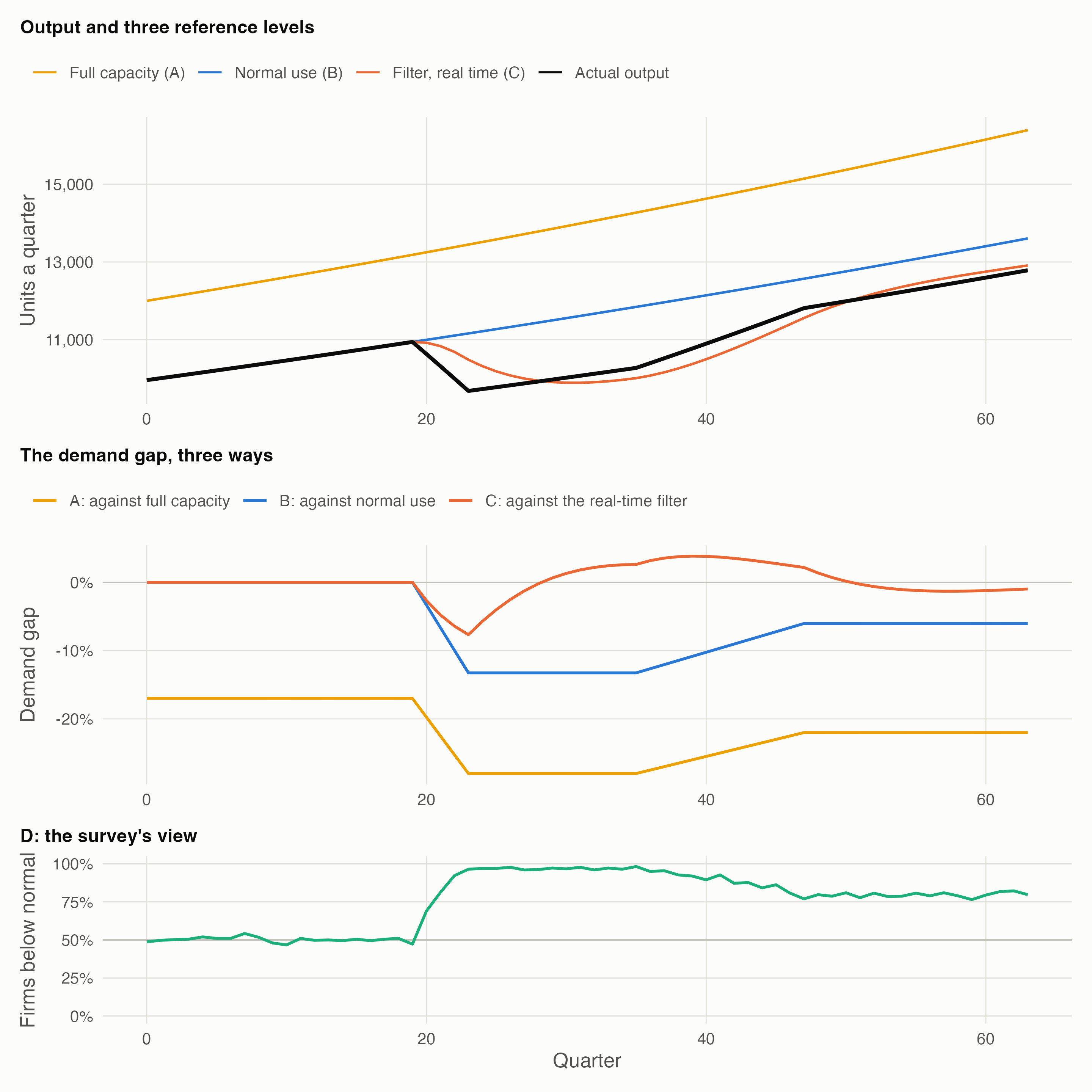
- A, engineering capacity, makes every quarter a shortage: −17% before the slump even starts, because firms keep spare capacity on purpose. It can’t tell a slump from a strategy, so it works as a ceiling, not as the reference for a gap.
- B, normal use, gives the clean reading: zero in normal times, −13% at the trough, and still −6% at the end, because output never fully recovered. It needs a view of firms’ normal rate, which UK surveys pin down only roughly.
- C, a statistical filter run in real time, sees a gap of −7.7% at worst, against −13% from normal use, and −1.0% by the end. The filter assumes potential is smooth and treats a lasting fall as partly a fall in potential, so the long shortfall is gradually relabelled as lower potential. During the recovery it even reads 3.8% of excess demand, while output is still well below firms’ normal.
- D, the survey, shows the share of firms below their own normal jumping from about half to 98%. It measures the sign and spread of B with no deflator involved, but not the size of the gap.
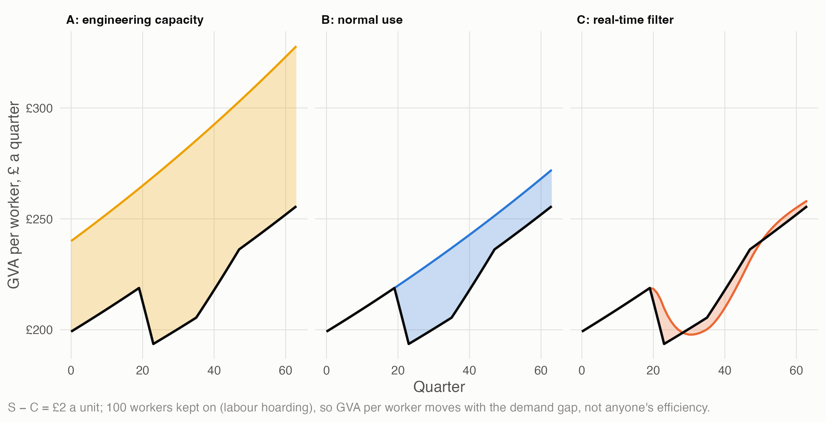
The same industry’s productivity, split four ways. With S − C = £2 a unit and 100 workers kept on through the slump, GVA per worker = potential productivity + the demand term, and where the line is drawn depends entirely on the meaning:
3 If potential adapts to demand
Post Keynesian economists argue over whether firms’ normal rate of capacity use is fixed or drifts towards whatever use they actually experience (the “utilisation controversy”). Mainstream filters build in a version of the same drift. So R5 recommends one switch for both: does potential adapt to actual output, and how fast?
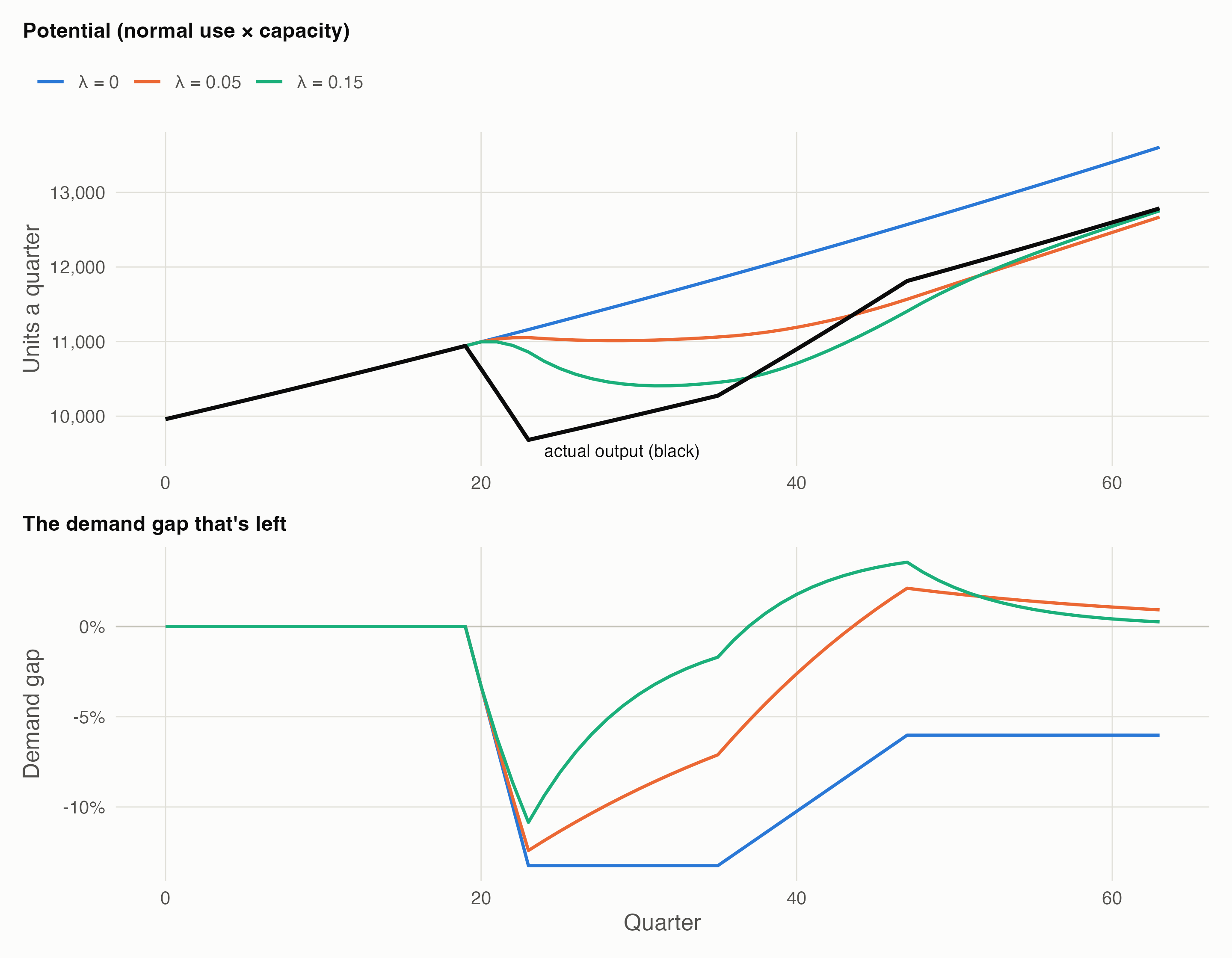
With no drift, the demand shortage is still −6% at the end. With firms’ normal drifting by 15% of the gap each quarter, it has closed (0.3%): the slump has been turned into lower “potential productivity”, and the demand aspect has disappeared from view. That is the disagreement between Webber’s reading and a supply-side reading, as one dial.
4 UK data
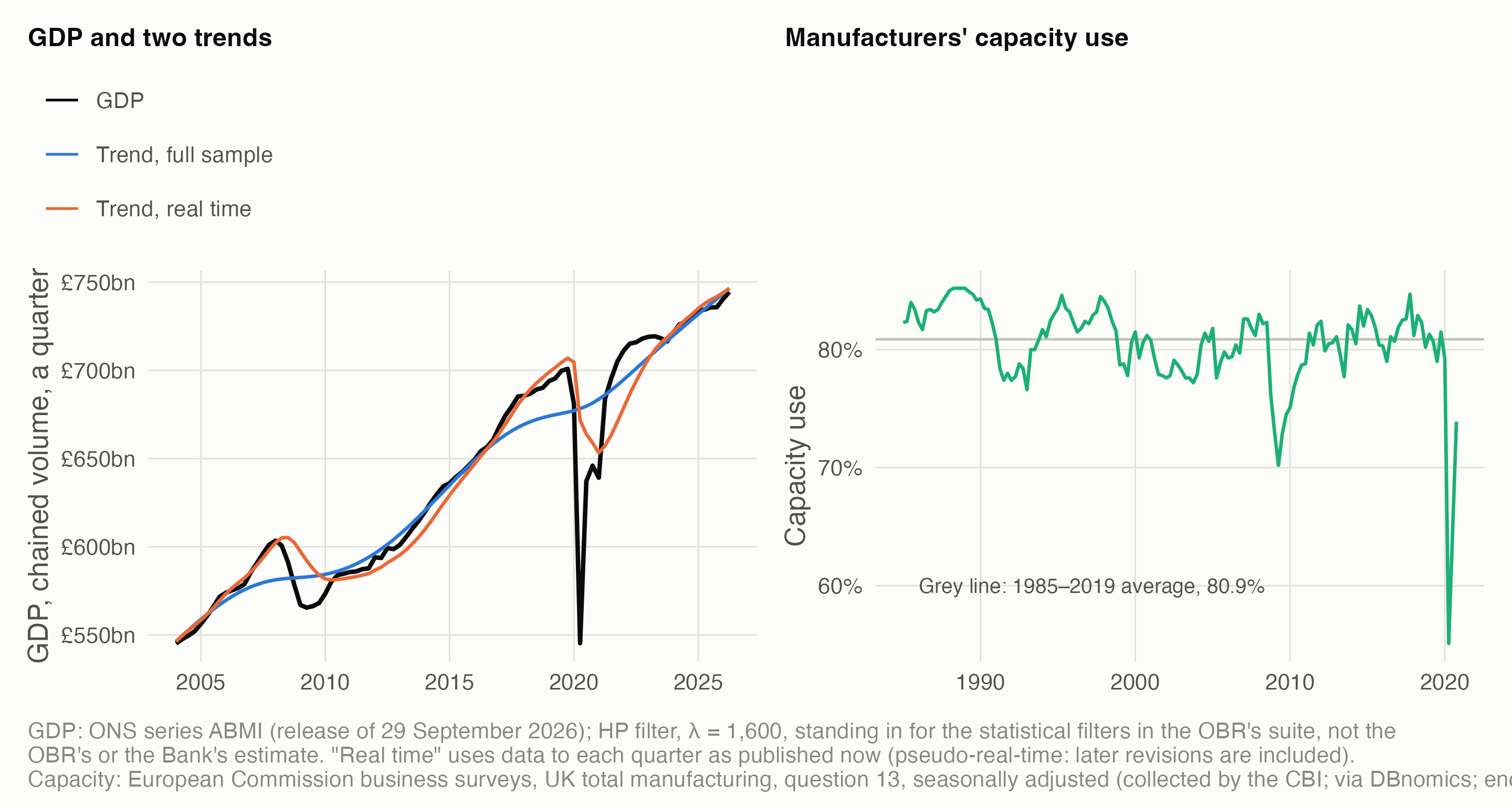
- The filter catches down. At the end of 2011, 2012 and 2013, the trend estimated with the data available at the time put GDP 0.5–1.5% above potential; fitted to the whole series, the same filter puts it 0.4–1.1% below. In real time, the filter had already re-read much of the post-2008 shortfall as lower potential, as in meaning C above; the OBR’s own working paper notes this end-point bias. It did the same in the pandemic: at the end of 2020 it read GDP as 2.0% below potential, against 5.2% with hindsight.
- Two cautions. This is a pseudo-real-time estimate, using today’s revised GDP; true real-time estimates, made with the data published at the time, would differ again. And large shocks distort the filter itself: fitted to the whole series, its trend bends down ahead of 2020, so it puts 2019 well above potential.
- Surveys anchor meaning B. UK manufacturers’ capacity use averaged 80.9% over 1985–2019. Read against that average, as the Bank and the OBR read their surveys, it measures normal use directly. The series stops in 2020; the CBI’s own survey continues under licence.
5 Footnote 20
The paper’s footnote 20, “This assumes there is inter-temporal redistribution”, qualifies its claim that higher wages that don’t cost other factors must come with higher S or Q. R5’s most plausible reading, with moderate confidence: the wage rise is paid out of the other parts of GVA first, and repaid later as the extra wages are spent and Q grows. That is Rowthorn’s “paradox of costs”, in the source the paper cites (Lavoie & Stockhammer, ILO 2012). It needs all firms to raise wages together, spare capacity and wage-led demand. A static rectangle can’t show it; two periods can.
6 Open questions
- Which meaning of potential should a model use, and should it adapt? R5’s recommendation, the working default: normal use (B) as potential, full capacity (A) as a ceiling, mainstream potential (C) as a switchable lens, surveys (D) as the data anchor, and one switch for adaptation speed. Decision 11 is still open.
- How do UK producer prices record a smaller pack at the same price? Only ONS’s business prices team can say. Asking them is the owner’s call.
- Footnote 20: only the authors can confirm the reading.
- Normal use by industry. The survey series here is manufacturing only and stops in 2020. Capacity is fuzzy in many services, and non-market output is measured by inputs.
Data and code. claude_research/productivity/R/c1_potential.R makes every figure’s numbers: the stylised industry and the adaptation runs (illustrative), the isoGVA curves, the HP filters on ONS series ABMI, and the European Commission survey series. Sources: Webber, D.J. & Huaccha, G. (2024) “Rethinking productivity: the crucial role of demand”, Journal of Post Keynesian Economics 47(1): 55–83; ONS methods documents for consumer, producer and services producer prices (as cited in R5’s note); OBR Working Paper 5 (2014); European Commission harmonised business surveys (via DBnomics). Full working: the Q5 frame and R5’s note.