Rising costs: demand or supply?
Telling the two apart: the identification problem, a simulation with a known answer, and UK tests
In short:
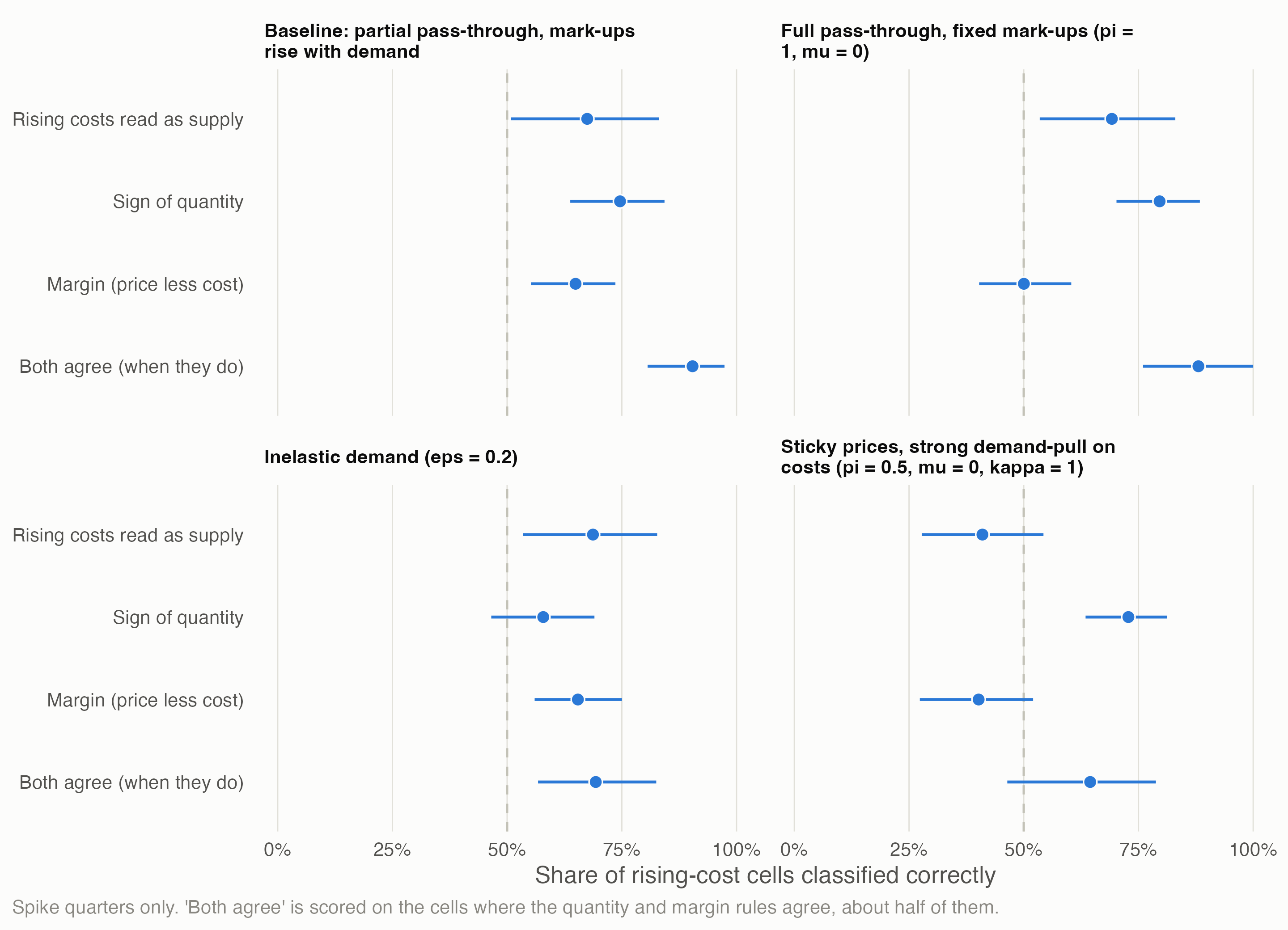
- Rising costs alone can’t tell demand from supply. A demand boom raises input costs as firms bid for inputs; an outside shock raises them directly. Firms will report “rising costs” either way. In a simulation where the true cause is known, reading rising costs as supply is right only 67% of the time.
- Adding what happened to quantities and margins helps, but each fails somewhere. The quantity sign is right 75% of the time and the margin 65%. When they agree they’re right 90% of the time, but they agree in only half the cases. Both fail in predictable conditions: inelastic demand, full pass-through, sticky prices.
- Variation that only one cause can produce does better. An outside cost shock that hits industries in proportion to their exposure recovers the true pass-through (instrumental variables: 0.81 against a true 0.80; plain regression: 1.21). It fails if demand moved with exposure.
- In UK manufacturing, the 2021–23 energy shock worked as a cost-push shock. Divisions that spend more of their output on energy raised prices more, by 5.9 log points per percentage point of energy intensity between 2019 and mid-2023 (5.5–6.4 leaving out any one division). Their volumes fell more, by 8.7 points per percentage point, and haven’t recovered.
- That identifies only the energy-driven difference between industries, not the common rise. How much of 2022–23’s general inflation was demand stays open.
The question comes from the Q4 pilot (page 5): in 2022–23 firms cited rising costs far more than shortages or weak demand, and whether rising costs count as a supply constraint decides the downturn. The owner’s view (decision 14): rising costs could signal either. This page treats that as an identification problem, in the sense of Huntington-Klein’s The Effect (2021, ch. 5), whose opening example asks why avocado prices fell while the quantity sold rose, and answers by asking which side of the market produced the variation. Script: claude_research/productivity/R/b1_rising_costs.R.
1 The problem
In The Effect’s terms:
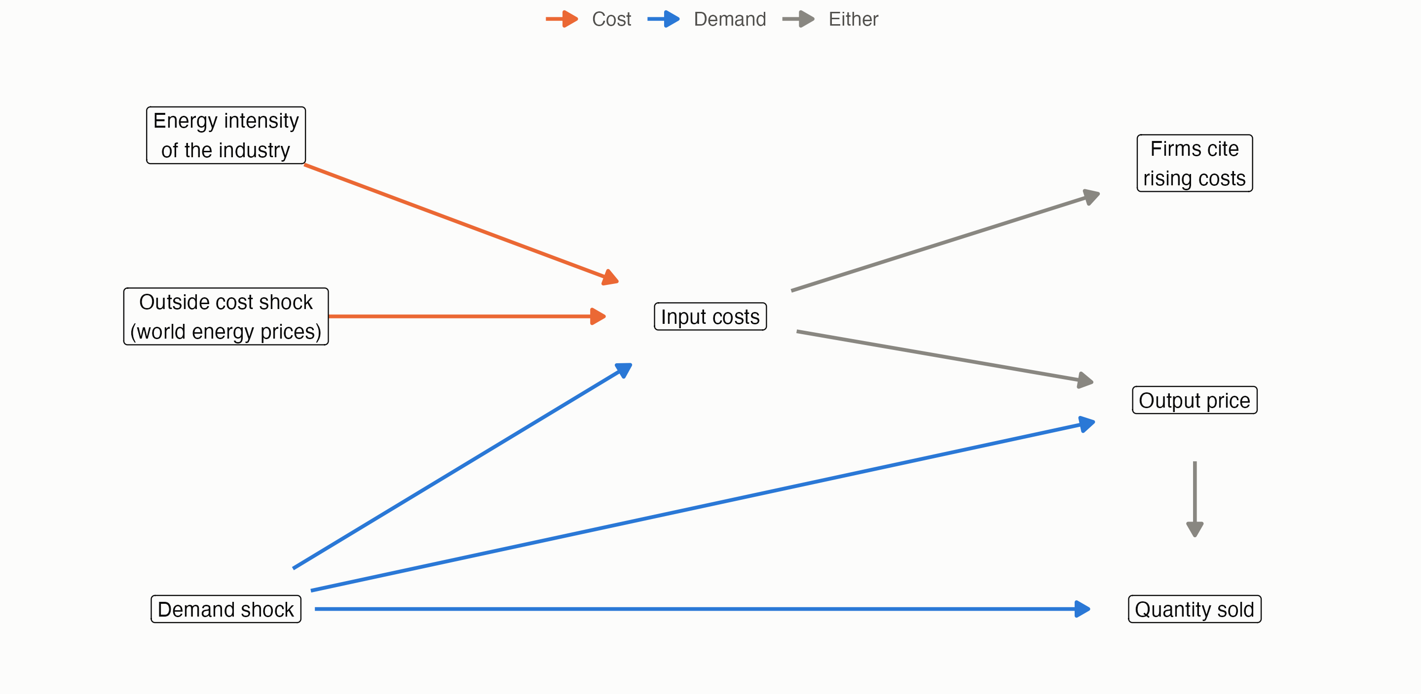
- The data-generating process. Input costs have two parents, a demand shock and an outside cost shock. “Firms cite rising costs” is a child of input costs, so it inherits both. Seeing it can’t say which parent moved.
- Where’s the variation? What separates the two routes is what they do downstream (quantity, the margin between price and cost) and what starts them (an outside shock whose size we can measure, hitting industries unevenly).
- Closing off alternatives. Each method below works by blocking one route, and each rests on an assumption that, if wrong, lets the other route back in.
2 A simulation with a known answer
As The Effect does with its simulated examples, the methods are first tried on data where the answer is known. Forty industries over 40 quarters, in log changes per quarter:
\[ \begin{aligned} \text{input costs} \quad c &= e\,z + \kappa\,d + \text{noise} \\ \text{output price} \quad p &= \pi\,c + \mu\,d + \text{noise} \\ \text{quantity} \quad q &= d - \varepsilon\,p + \text{noise} \end{aligned} \]
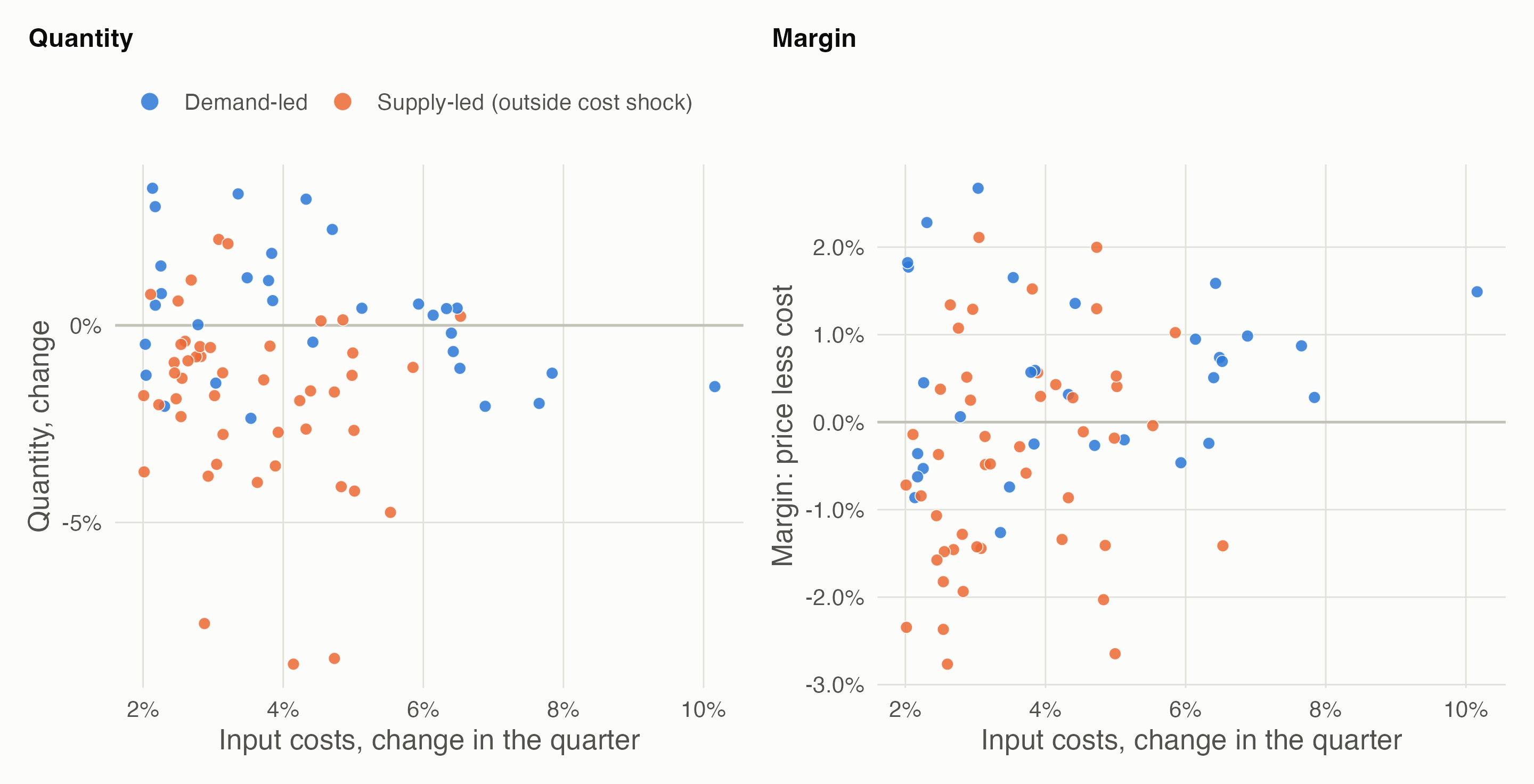
Here z is an outside energy-price shock (with a four-quarter spike, like 2022), e each industry’s energy intensity (2–25% of costs), d an industry demand shock, κ how far demand pulls up input costs, π cost pass-through, μ how far demand raises mark-ups, and ε the price elasticity of demand. A cell where costs rise is supply-led if e z exceeds κ d. Baseline: κ = 0.5, π = 0.8, μ = 0.3, ε = 1.
What each rule assumes, and when it fails:
- “Rising costs mean supply” is right exactly as often as supply-led cells are common: 67% in the baseline. It’s a guess about the mix, not evidence.
- The quantity sign (costs up and quantity down means supply) assumes demand is elastic enough for a cost shock to cut sales. With inelastic demand it drops to 58%.
- The margin (costs up and the margin squeezed means supply) assumes pass-through is incomplete and that demand raises mark-ups. With full pass-through and fixed mark-ups it falls to 50%. With sticky prices and strong demand-pull on costs, demand squeezes margins too, and the rule is right only 40% of the time.
- Both together are right 90% of the time when they agree, but abstain on about half the cells. Disagreement is itself the honest answer there.
Using variation only one cause can produce. The outside shock z hits industries in proportion to their energy intensity e, and demand doesn’t (in the baseline). So e × z moves costs for supply reasons only:
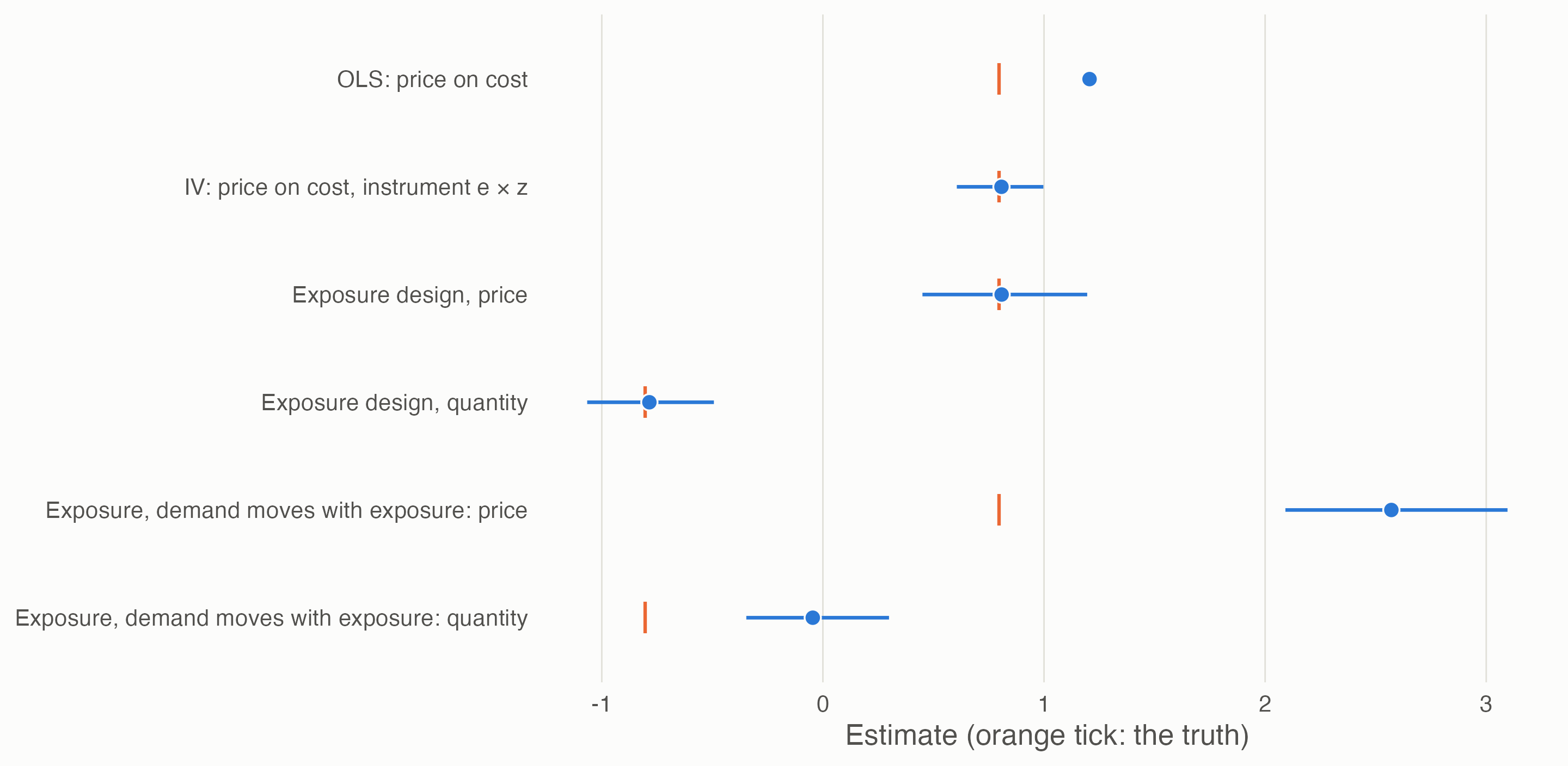
- Instrumental variables recover pass-through. Regressing price on cost gives 1.21, because demand raises both; using only the cost variation driven by e × z gives 0.81, against a true 0.80. This needs the instrument to move costs (relevance) and to touch prices and quantities only through costs (exclusion).
- The exposure design (difference-in-differences, or an event study, with exposure as the “dose”) recovers both the price and the quantity response. Its key assumption is that, absent the shock, more and less exposed industries would have moved alike (parallel trends). If demand also moved with exposure, the price response is overstated (2.57) and the quantity response all but vanishes (−0.05).
3 Approaches, side by side
| Approach | The variation it uses | It assumes | It fails when | UK data |
|---|---|---|---|---|
| Firms’ stated reasons | Survey answers (“rising costs”) | Firms can tell why costs rose | Costs rise for both reasons | BICS, CBI, BCC |
| Price–quantity signs (Shapiro) | Surprises in price and quantity | One shock dominates each period | Shocks are mixed; ρ is small (page 5) | Producer prices, GDP(O) volumes |
| Signs with a third variable | Costs and the margin as well | Incomplete pass-through; mark-ups move with demand | Full pass-through; sticky prices | Input and output price indices, supply and use deflators |
| Exposure design (DiD, event study) | Industries hit harder by an outside shock | Parallel trends; exposure measured before the shock | Demand moves with exposure | Supply and use tables (exposure); prices and volumes |
| Instrumental variables | Cost changes driven by exposure × shock | Relevance and exclusion | The shock also moves demand (energy prices cut real incomes) | As above, plus world energy prices |
| Narrative and policy events | Dated shocks of known direction | The event is the only thing that changed | Other shocks coincide | Eat Out to Help Out (Aug 2020, demand); Energy Bill Relief Scheme (Oct 2022, costs) |
| External instruments in a VAR | Shocks identified elsewhere (oil supply news; monetary policy surprises) | The external series is exogenous | Weak instruments; UK series to build | Published shock series; quarterly industry data |
| Bayesian priors on elasticities (Baumeister & Hamilton) | Plausible ranges for supply and demand slopes | The priors are honest | Priors drive the answer | Literature ranges |
One general caution, from the frame: the energy shock also cut real incomes, so an outside cost shock can lower demand for other industries. That breaks the instrument’s exclusion and the clean split into “demand” and “supply” at the same time. Shocks are often both.
4 UK tests
4.1 The 2022 energy shock across manufacturing
Design. Exposure = each manufacturing division’s purchases of electricity, gas and refined fuels as a share of its output in 2019, before the shock (Blue Book 2026 supply and use tables). It runs from 0.5% to 5.5%, highest in non-metallic minerals, chemicals and paper. Outcomes: domestic output producer prices and chained-volume GVA, as changes from their 2019 average, before both Covid and the energy shock (wholesale gas prices began rising in 2021). For each quarter, the change is regressed on exposure across 21 divisions; the coefficient is the extra change per percentage point of energy intensity. Common shocks, demand or cost, fall into the intercept and are not attributed. Refining (C19) is left out: it supplies energy rather than buying it.
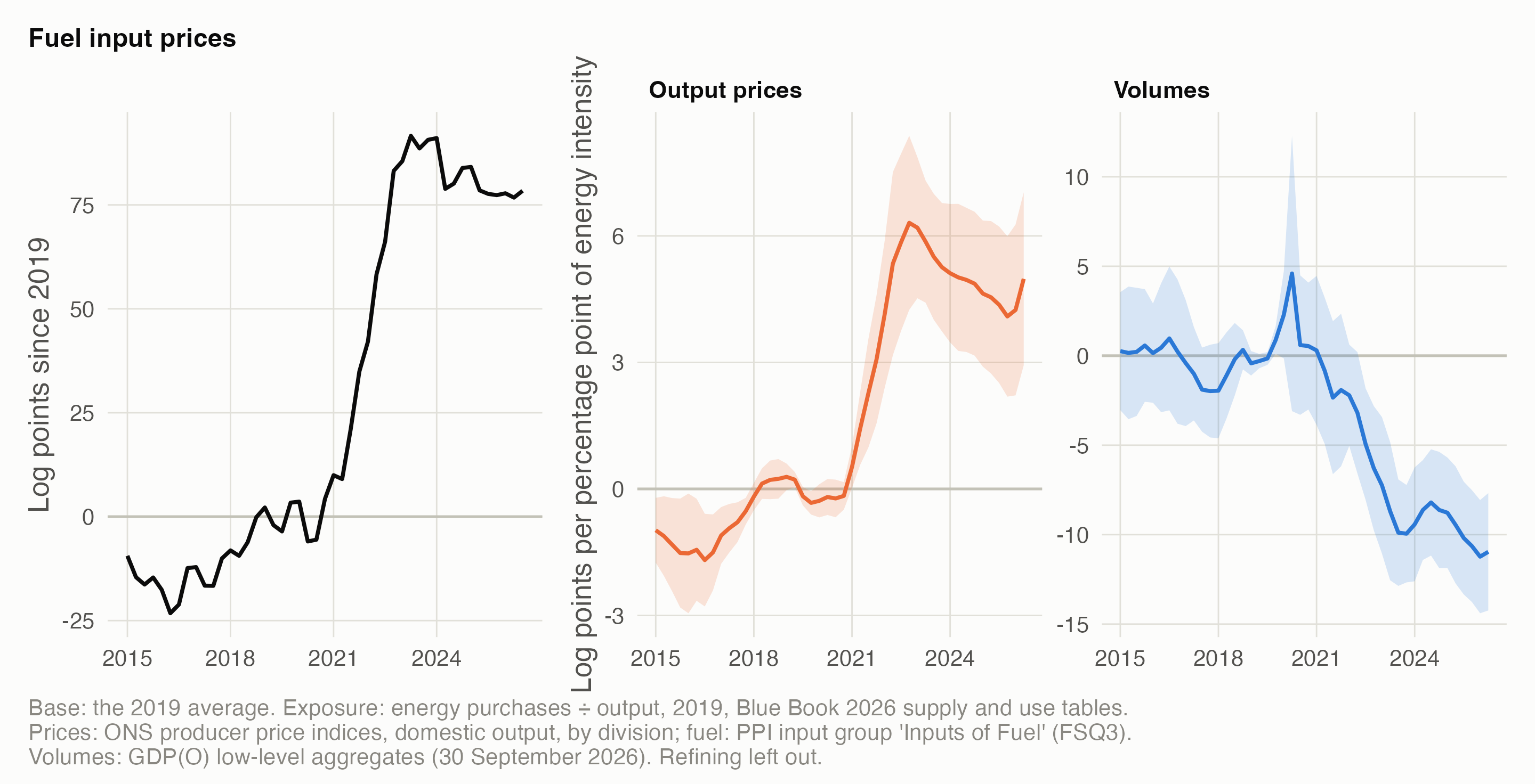
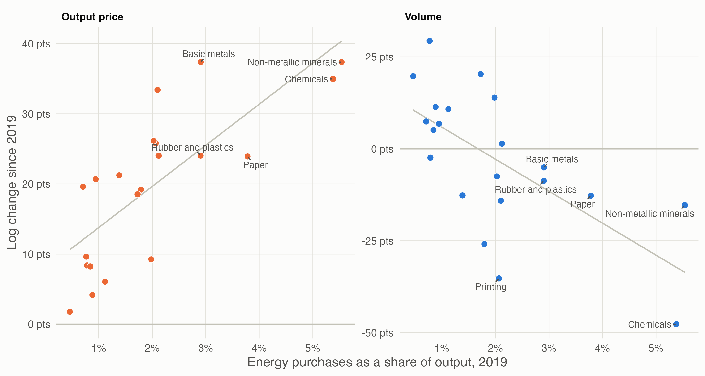
- Prices: a clear dose–response, timed with energy prices. By mid-2023 each percentage point of output spent on energy came with 5.9 more log points of price rise since 2019 (5.5–6.4 leaving out any one division). The coefficient peaked at 6.3 in 2022 Q4 and has eased to 5.0 by 2026 Q2, even though fuel prices stayed high.
- Volumes: a lasting loss. Volumes fell 8.7 more points per percentage point by mid-2023 (6.8–11.1 leaving one out), and the gap has kept widening, to 11.0 by 2026 Q2.
- The pre-trend check is imperfect, in an informative way. Before 2019 the price coefficient drifted by up to 1.7 points, when fuel prices were also moving (about 10–15% below their 2019 level in 2015–17). So exposure always matters when energy prices move: that supports the mechanism, but there’s no shock-free baseline. The volume coefficients sit near zero before 2021, apart from Covid noise in 2020.
- Reading: for the energy-driven part, the rising costs of 2021–23 in manufacturing behaved like a supply shock: prices up and volumes down in proportion to exposure, with the volume loss persisting. It says nothing about the common rise all divisions shared, which could be demand, wages or supply chains.
4.2 The margin test across the pilot’s industries
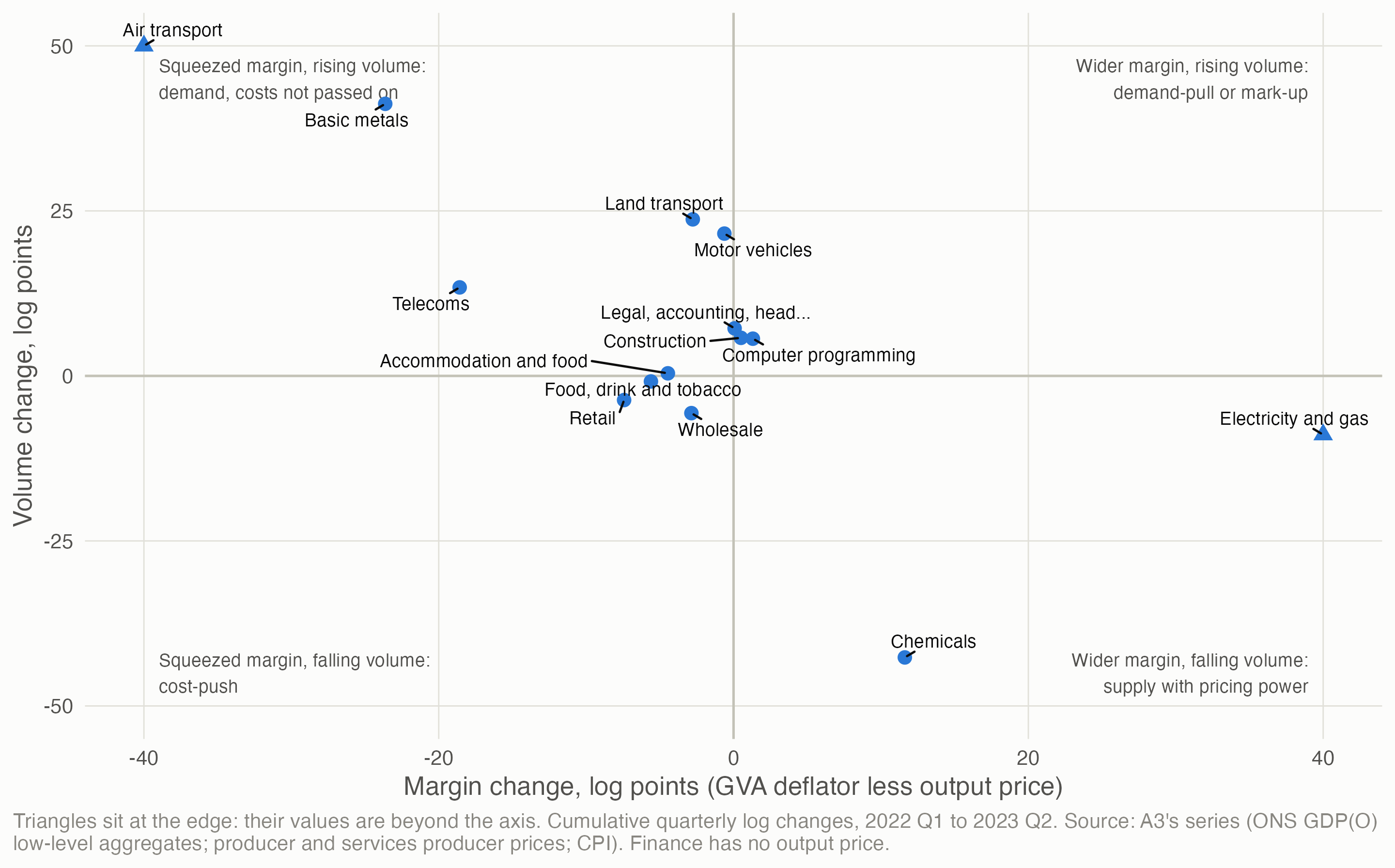
What it shows, and why to be careful. Food manufacturing, wholesale and retail sit where a cost-push shock would put them: margins squeezed, volumes down. Electricity and gas shows margins widening as volume fell, the energy windfall that page 3 finds in its excess. But the margin here uses the implied GVA deflator, and for several industries (air transport, basic metals, chemicals) the numbers are dominated by post-pandemic recovery or by how ONS derives the deflator: the division bias that page 5 found. The margin test needs observed input prices by industry, which ONS doesn’t publish directly.
5 What this means for 2022–23
- Don’t settle “rising costs” by fiat. Counting them as supply or as demand in the pilot’s survey signal would each be wrong much of the time; the simulation suggests about a third of the time in a mixed episode.
- The energy shock’s own footprint was supply-side, at least across manufacturing: prices rose with energy intensity, and volumes fell. Firms’ “rising costs” in energy-intensive sectors are best read as cost-push.
- The common part is unidentified. Every division’s prices rose, and the exposure design can’t say why. Demand recovery, wages and supply chains all remain candidates.
- For the pilot, a third survey reading becomes defensible: “costs, energy-driven” (supply) where exposure is high, “costs, unattributed” elsewhere. That rule would be chosen after seeing results, so it would have to be labelled that way.
6 Open questions
- Beyond manufacturing. Services have fewer price indices and less exposure variation. Transport (fuel) and hospitality (energy and food) are the obvious next cases.
- Input costs by industry. Building each industry’s input price index from the supply and use tables’ input mix and ONS’s product input prices would make the margin test direct, and is how ONS itself double-deflates.
- Two instruments, two shocks. World energy prices for the cost side and something like UK monetary policy surprises for demand, in one framework, would separate the common part too.
- Policy events. The Energy Bill Relief Scheme (October 2022) cut business energy costs without a demand impulse: a test of pass-through in reverse.
- Firm-level data (BICS microdata in the Secure Research Service) would let exposure vary between firms, not just industries.
Data and code. claude_research/productivity/R/b1_rising_costs.R runs the simulation (200 panels per scenario), the UK event study and the margin test. Sources: ONS supply and use tables, Blue Book 2026 (30 October 2026); ONS producer price indices (vintage of 21 October 2026); ONS GDP(O) low-level aggregates (30 September 2026); A3’s industry series (page 5). Method: Huntington-Klein, N. (2021) The Effect: An Introduction to Research Design and Causality, ch. 5 “Identification”; Shapiro (2022); Read (RBA 2024); Baumeister & Hamilton (2019), as reviewed in R4’s methods note.